A boat approaching a quay must arrive in the right place, face along the berth, and lose its remaining momentum. A sequence of thrust commands determines all three outcomes. The shooting formulation turns this task into an optimization over those commands: simulate a candidate sequence, measure its cost, and improve it. How can an optimizer use the time structure of the simulation when computing that improvement?
Linearizing the dynamics along the current trajectory and quadratically approximating its costs gives a problem whose controls can be eliminated backward, one time step at a time. The resulting correction is then tested through the nonlinear simulator. Repeating these operations gives the iterative linear-quadratic regulator, or iLQR. Keeping additional curvature from the dynamics gives differential dynamic programming, or DDP. Both methods compute corrections around a nominal trajectory. Their backward recursions follow from substitution and quadratic minimization.
Learning Goals
After working through the derivations and examples, you should be able to:
Construct a local quadratic optimal-control problem around a feasible rollout.
Eliminate its controls backward and recover an affine correction at each step.
Implement nonlinear trial rollouts with line search and regularization.
Identify the dynamics-curvature terms that distinguish DDP from iLQR.
Assess a docking plan using its cost, arrival velocity, and hull clearance.
Explain how thermal load and nonlinear power loss shape a bounded cooling schedule.
Prerequisites
The chapter uses the finite-horizon optimal-control formulation, single shooting, and first and second derivatives. The sequential-methods discussion introduces general SQP subproblems, and the initial-value-problem appendix reviews numerical integration. Neither dynamic programming nor a previous derivation of LQR is required.
A Docking Problem
Docking requires the boat to reach the berth, align with the quay, and shed its momentum. A trajectory that reaches the right position with appreciable translational or angular velocity will carry the boat away again.
Consider a two-metre boat moving in the horizontal plane. Its state and control are
The position and velocity are measured in fixed world coordinates, is the heading, and is the angular velocity. Each control is a fraction of maximum thrust. Positive commands push forward and negative commands push backward. Unequal thrusts turn the boat. There is no directly commanded sideways force, so an approach with sideways momentum requires a maneuver.
Let point along the boat and point across it. The simplified inertial model is
The drag opposes velocity along each boat axis, with stronger resistance to sideways motion. Thrust changes acceleration, so releasing the controls does not stop the boat immediately. These equations are a synthetic teaching model for calm water, with neither contact forces nor waves.
| Quantity | Value |
|---|---|
| Mass | |
| Angular inertia | |
| Thruster lever arm | |
| Maximum force per thruster | |
| Longitudinal drag | |
| Lateral drag | |
| Angular drag | |
| Rectangular hull length and width | , |
The quay occupies , and the desired arrival state is . The boat should lie parallel to the quay with its center one metre from the edge. The angled approach starts from . The sideways-drift case changes only to . Angles are in radians. Both experiments use piecewise-constant controls, each held for , for a total of 20 seconds. Thus is the initial state and is the arrival state, as in the preceding chapters. One fourth-order Runge--Kutta step gives for .
To discourage the hull from approaching the quay, let be the world-coordinate height of rectangular corner . With a desired buffer and smoothing length , define
This is a smooth penalty for violating the buffer. Its finite weight permits violations, so the final trajectories will also undergo a separate geometric clearance check. The full rectangle is used for that check, including the area outside the pointed boat icon in the figures.
For , the running and terminal costs are
These numerical weights apply to the stated SI coordinates and dimensionless thrust commands. The periodic heading penalty assigns the same cost to angles that differ by a full turn. The simulator retains an unwrapped angle; it does not insert a discontinuity at into the differentiated transition.
The initial control sequence is zero, so the boat coasts and slows under drag. It stops far from the berth. Successive control updates can first bring it closer and then adjust the arrival heading and velocity.
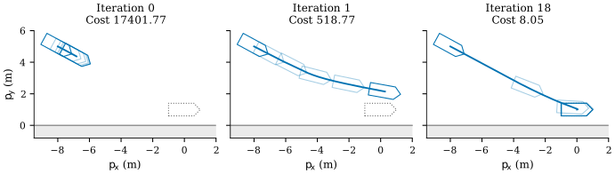
Figure 1:Accepted iLQR iterates for the angled approach. Every curve is a nonlinear rollout from the same initial state. Boat outlines are spaced four seconds apart; their overlap indicates slow motion. The dotted outline marks the desired berth. The first update reduces the position error substantially, while later updates refine the turn and stopping maneuver.
Taylor Models of Dynamics and Cost
The local model describes the change in cost caused by a small change in the thrust sequence. Start from the finite-horizon problem
Here is the complete control sequence. Its rollout determines every later state.
Set aside the control bounds while deriving the local correction. Roll out a nominal control sequence to obtain states satisfying . For a nearby trajectory, write and , and stack them as . Taylor expansion of the discrete transition at the nominal state and control gives
Subtracting and dropping the quadratic remainder gives the linearized dynamics . Both rollouts start from the same state, so . There is no constant defect because the nominal trajectory satisfies the discrete dynamics. Independently chosen state guesses would generally leave such a defect. We write for the combined Jacobian.
Taylor expansion of the running cost to second order gives
Here and ; the other gradient and Hessian blocks are evaluated at the same nominal pair. We denote the stacked gradient by and the displayed block Hessian by . Gradients are column vectors, matching the convention of the preceding chapters. We retain the linear terms: individual stage gradients need not vanish even at an optimal trajectory because the dynamics couple stages, and at a non-optimal nominal trajectory they also drive its correction. The block measures how the marginal cost of a control changes with the state. Even if the running cost has no such cross term, eliminating later controls can create one in the quadratic tail.
The terminal cost has the same expansion, with no control coordinate:
Dropping the remainders in these Taylor expansions yields a quadratic cost subject to linearized transitions. The state at one step couples only to its neighbors. This is the local problem solved by backward elimination. A general SQP method also forms local quadratic subproblems, but its exact Lagrangian Hessian includes terms from dynamics curvature. Those terms enter below when we develop DDP.
Backward Elimination
The last control affects only its own stage and the terminal state when its starting state is fixed. Eliminating it first leaves a shorter quadratic problem of the same form. Repeating that step works backward through the horizon.
A two-step calculation
Consider a scalar example with , initial state , dynamics , and cost
Treat as given while eliminating . Substitution of gives
Differentiating with respect to gives , so . Substituting this expression back into the last two terms of the cost leaves . Since , the remaining problem is
Its derivative is , giving . Forward substitution then gives , , , and . The final position is short of one because the objective trades terminal error against effort; arrival was penalized, not imposed as an equality.
The expression also carries information that a single number would discard: if the state reaching the last step changes, the minimizing last control changes with it. This dependence becomes the matrix feedback correction in the general calculation.
Eliminating a vector control
Suppose all controls after time have already been eliminated from the local problem. Write the remaining quadratic tail as
At the terminal step, is the quadratic Taylor polynomial of , so and its other coefficients are the defined above. At earlier steps, is obtained by elimination from a finite optimization problem. This construction does not require a function over all states of the nonlinear system.
Substitute into this tail and add the stage cost. With , the new linear and quadratic coefficients are
We use for the local Hessian because denoted the Hamiltonian in the Pontryagin chapter. Partition and according to the state and control coordinates. Apart from a constant, the expression to minimize is
The time index is suppressed within this one-step calculation. When is positive definite, setting the control derivative to zero gives
where
Restoring the time index gives the affine correction . The vector changes the nominal command even at zero state deviation. The matrix adjusts that change for a different state arriving from the earlier steps. In code, these formulas are linear solves with ; an explicit matrix inverse is unnecessary.
Substituting the minimizing control back into the quadratic expression gives the coefficients needed by the preceding step:
The subtracted term in is the Schur complement associated with eliminating the control block. Repeat this operation from to one, starting with the terminal coefficients. A subsequent forward substitution recovers the state and control changes. For fixed state and control dimensions, the number of these elimination steps grows linearly with the horizon.
For linear dynamics and quadratic costs, this procedure solves the original unconstrained problem exactly when its control minimizations are well posed. That problem is called the linear-quadratic regulator problem, and the matrix recursion for is a Riccati recursion. Along a nonlinear trajectory, , , and the cost derivatives describe only a local approximation. They must be recomputed after the trajectory changes.
Nonlinear Rollouts and iLQR
The backward pass minimizes a quadratic approximation. A large correction can make its linearized state prediction inaccurate, so a proposed control sequence must be evaluated through the original discrete simulator before it is accepted.
Starting from the same initial state, form a nonlinear trial trajectory using
The step size scales the feedforward change. The feedback term responds to the state deviation that actually occurs during this trial. Its gain is not multiplied by . At , induction through these equations recovers the nominal trajectory, because each state deviation is then zero. For an exact linear-quadratic problem, gives the complete solution derived by elimination.
A line search first tries , then successively smaller values. Each trial has its own nonlinear states and cost. The implementation uses and accepts a strictly lower finite cost with a small sufficient-decrease check. If
the backward pass estimates a reduction . Acceptance requires as well as a strict decrease. This estimate guides acceptance; it does not replace evaluation of the original objective.
The control curvature may be indefinite or nearly singular. Replace the matrix used in the control solve by , where . Increasing makes the correction more conservative and can make the solve positive definite. The code checks a Cholesky factorization, increases after a failed backward pass or line search, and decreases it after an accepted step. The numerical defaults start at 10-4, multiply by ten after failure, and divide by three after acceptance, with a floor of 10-9.
When regularization changes and , the simplified Schur-complement formulas above no longer describe substitution into the original quadratic model. The implementation therefore uses the full expressions
Here is the original curvature block; regularization was used to choose the correction. These expressions also remain applicable when some controls are fixed at their bounds.
Alternating local linear-quadratic approximation, backward elimination, and nonlinear rollout gives iLQR Li & Todorov, 2004. The iteration uses second derivatives of the costs but only first derivatives of the dynamics. It is often described as a Gauss--Newton approximation to DDP. That terminology should not obscure what is approximated: the omitted terms come from dynamics curvature. If a nonlinear cost is itself a sum of squared residuals, replacing its Hessian by a residual-Jacobian product would be a further approximation; the docking code uses the exact cost Hessian.
The returned gains describe a neighborhood of the final nominal trajectory. The docking animation below executes one stored plan. The gains used inside the optimizer do not imply that the animation replans as the boat moves.
Dynamics Curvature and DDP
iLQR drops the quadratic remainder in the transition’s first-order Taylor expansion. For a turning boat, a change in heading changes the direction of thrust, so products of state and control changes can affect the next state. DDP retains these second-order terms in the backward calculation.
For component of the transition, Taylor expansion one order further gives
Here is the Hessian of the th component of with respect to the stacked state and control, evaluated at the nominal pair. Substitute this expression into the same quadratic tail . Its linear term now contributes an additional quadratic term. Its quadratic term contributes ; products involving the second-order part of the transition there are of order three or higher and are discarded. Consequently,
The extra contraction weights curvature of each next-state component by its linear coefficient in the eliminated tail. At a given backward stage, this is the second-order chain rule for composing the transition with that tail. In block form, the differences from iLQR are
Setting those three sums to zero recovers the iLQR construction. Retaining them and using the same quadratic elimination and nonlinear line search gives DDP Tassa et al., 2014. The two methods share an algorithmic structure; the curvature choice can change both the direction of a step and the amount of regularization needed to accept it. This derivation does not require solving a subproblem with quadratic dynamics constraints.
For the boat, even the continuous acceleration contains a state--control cross derivative: . The discrete derivatives used by the solver also include how heading and velocity change within the RK4 step. Automatic differentiation is applied through that complete step. A differential equation that is affine in its controls need not yield a numerical transition whose second control derivatives vanish.
The extra curvature costs computation and can be indefinite. DDP therefore still needs regularization and nonlinear acceptance tests. Neither method guarantees the globally best docking maneuver. For affine dynamics the transition Hessians are zero, so the two backward constructions coincide when all other choices agree.
Thruster Limits and Stopping Criteria
The boat’s controls must remain in , even when the unconstrained correction asks for more thrust. At zero state deviation, the feedforward step is the solution of the box-constrained quadratic problem
For two controls, each coordinate is either free, fixed at its lower bound, or fixed at its upper bound. The teaching implementation checks the nine combinations, minimizes over each face, and keeps the best feasible candidate. Positive-definite curvature makes this a strictly convex QP. Larger systems can use an active-set solver rather than enumerate all combinations Tassa et al., 2014.
The feedback rows of saturated controls are zero while their active set stays fixed. For the free coordinates , solve . Use the full substitution formulas to update the quadratic tail. With bounds, this tail describes a neighborhood with the selected active sets; across active-set changes the minimized expression is generally piecewise quadratic. During the nonlinear trial, project the resulting control onto its box before simulation. This enforces the physical bounds when a trial leaves the neighborhood represented by the backward pass. The nonlinear cost check then decides whether that trial should be retained.
The stopping test is separate from docking success. Let be the gradient of the original shooting objective, computed by the adjoint recursion along the current nonlinear rollout. With normalized controls, the solver stops when
At an interior optimum this reduces to a small control gradient. At a bound it also allows a gradient that points toward a forbidden improvement. The experiment permits at most 120 accepted updates. If regularization exceeds 1012 without an acceptable trial, the solver retains its last accepted trajectory and reports failure to make progress. A small residual certifies approximate first-order stationarity, not a globally optimal path or a successful arrival.
Docking Trajectories and Recorded Futures
Do the two curvature choices produce the same maneuver from the same starting plan? Both methods receive the coasting initialization, identical costs and control limits, and the same stopping settings. The following tables report their final nonlinear costs and arrival checks. Each final control sequence is also replayed with four RK4 substeps per control interval, giving a validation grid.
| Approach | Method | Cost | Accepted updates |
|---|---|---|---|
| Angled approach | iLQR | 8.0515 | 18 |
| Angled approach | DDP | 11.9879 | 34 |
| Sideways drift | iLQR | 7.6674 | 13 |
| Sideways drift | DDP | 7.6674 | 45 |
The arrival checks below use the finer replay.
| Approach | Method | Position error (m) | Heading error (°) | Speed (m/s) | Clearance (m) |
|---|---|---|---|---|---|
| Angled approach | iLQR | 0.000125 | 8.98e-05 | 6.89e-05 | 0.599 |
| Angled approach | DDP | 0.00125 | 0.139 | 0.0144 | 0.352 |
| Sideways drift | iLQR | 3.89e-05 | 2.65e-06 | 4.25e-05 | 0.600 |
| Sideways drift | DDP | 3.89e-05 | 3.71e-06 | 4.25e-05 | 0.600 |
All four runs satisfy the stopping test and the docking checks: position error below , heading error below , speed below , angular speed below , bounded thrust, and positive hull clearance. The maximum position difference between the planning trajectory and the finer replay is below in these runs. Clearance is checked on the finer grid; this remains a sampled validation, not a proof of continuous-time collision avoidance.
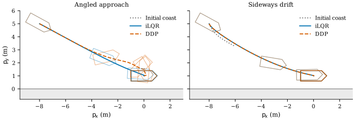
Figure 2:Final trajectories under the same initialization and objective. Solid blue is iLQR and dashed orange is DDP; the dotted gray path is the initial coast. Outlines show orientation every four seconds. DDP takes a different turning maneuver in the angled approach. The two final paths nearly coincide in the sideways-drift case.
In the angled approach, iLQR reaches cost 8.0515 in 18 accepted updates, while DDP reaches a different stationary trajectory with cost 11.9879 in 34 updates. The DDP trajectory makes two full turns near the berth. Its final unwrapped heading is approximately , which the periodic heading cost treats as the same orientation as zero. Reaching this stationary trajectory does not remove the extra motion accumulated on the way there. In the sideways-drift case, both reach cost 7.6674, with 13 accepted updates for iLQR and 45 for DDP. These are outcomes of two particular local solves, not a general ranking of the algorithms. The difference in the first case also shows why comparing iteration counts alone can hide a difference in the solutions obtained.
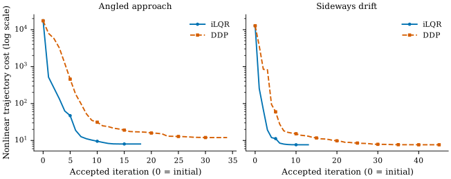
Figure 3:Actual nonlinear cost at every accepted iteration, including the initial rollout at iteration zero. The vertical axis is logarithmic. Rejected trial steps are excluded from the horizontal count; forward-evaluation and backward-attempt counts are available in the downloadable diagnostics.
Within one selected plan, simulation time has a different meaning from optimizer iteration. At two seconds, for example, the boat occupies the two-second state of that rollout. Its remaining states give a prediction of where it will go if the rest of the stored controls are applied. Outlines spaced equally in time spread apart while the boat is moving quickly and cluster as it comes to rest. Reverse thrust helps remove momentum before arrival.
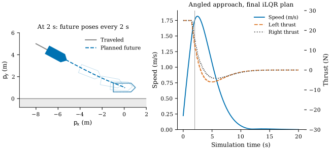
Figure 4:The final iLQR plan for the angled approach. The filled boat marks the selected simulation time; translucent outlines show future poses every two seconds. The right panel gives speed and both physical thrusts. Negative thrust during the approach brakes the boat. The vertical marker identifies the same time as the filled boat.
Choose a scenario and optimizer iteration, then scrub or play simulation time within that fixed plan. The path ahead and boat outlines display its remaining predicted states. Arrival errors and plots belong to the selected iteration, including intermediate plans that do not dock successfully.
The replay reads recorded simulations, so exploring it does not rerun an optimizer. Recomputing a plan from newly observed states is the additional step introduced in receding-horizon control.
Pulling Down a Thermoacoustic Refrigerator
A standing-wave thermoacoustic refrigerator is a sealed, gas-filled tube with a loudspeaker at one end and a stack of thin parallel plates inside (Figure 6a). The loudspeaker excites a standing sound wave in the tube. Each gas parcel near a plate is pushed back and forth along it, compressing and heating as it moves toward the loudspeaker end and expanding and cooling as it moves away. At the loudspeaker end of its travel the parcel is warmer than the plate and gives up heat to it; at the far end it is cooler than the plate and takes heat from it. Every cycle therefore moves a little heat one step along the plate, and the parcels together act as a bucket brigade that transports heat from the far end of the stack toward the loudspeaker end. Sound is used to move heat from a cold place to a warmer one, against the direction it would flow on its own. A household heat pump does the same thing with a compressor when it extracts heat from cold outdoor air and delivers it indoors; a refrigerator is the same machine used for its cold side. A cold heat exchanger at the far end of the stack connects to the payload, the refrigeration term for the object or compartment being cooled, and a hot heat exchanger at the loudspeaker end rejects the heat to ambient air. There are no moving parts other than the loudspeaker, and the only knob is how hard it drives. The control problem is what refrigeration engineers call a pull-down: bringing the payload from ambient temperature down to its set point after switch-on. Here that means choosing a driver-amplitude schedule that brings the payload to a target temperature by a fixed deadline while spending little acoustic energy.
Figure 6:Geometry of the thermoacoustic refrigerator and its two-state abstraction. (a) The device: a loudspeaker piston at the left end of a sealed resonator, a hot heat exchanger, a stack of thin plates, and a cold heat exchanger. The dashed envelope is the standing-wave pressure amplitude. Gas parcels oscillating along the plates pump heat from the cold exchanger toward the hot one. (b) The lumped model the optimizer sees. The state is the pair of exchanger temperatures, the action is the driver amplitude, the stage cost charges acoustic work, and the terminal cost penalizes the final cold-side temperature error. In the online book the figure replays the recorded iLQR and DDP plans: the piston stroke, wave, and parcel motion follow the action, the exchanger and node tints follow the state, and the panels below compare the plan with a constant-amplitude schedule. The static version shows the same two panels.
In the online book, the replay reads the recorded plans and integrates only the constant-amplitude comparison; it does not rerun the optimizer.
Rather than simulate the acoustics, we lump the whole device into two thermal masses (Figure 6b): the cold exchanger together with its payload, and the hot exchanger. The state is their temperatures, , and the action is the normalized driver amplitude , so this is a two-dimensional continuous-state, one-dimensional continuous-action problem. Let be the temperature span across the stack and a pumping efficiency that decreases linearly with that span. The continuous-time dynamics are
Here is the heat pumped out of the cold side, is the acoustic work the driver injects, is a parasitic heat leak into the payload, and is the hot exchanger’s conductance to ambient. Both heat flows scale with because acoustic power is quadratic in wave amplitude, and both weaken as the span grows; this is the short-stack approximation of thermoacoustics Swift, 1988Swift, 2017. Two loss terms complete the work: a viscous term in and a cubic term that makes hard driving disproportionately expensive. The coupling matters for the optimizer. Driving hard pumps heat faster, but it also dumps that heat plus the work into the hot side, which raises , widens the span, and lowers the efficiency of every later step. Refrigeration engineers measure this efficiency by the coefficient of performance (COP), the ratio of heat pumped to work spent while the driver is on. Unlike an efficiency it can exceed one, because the work only moves heat rather than producing cold. In this model the COP falls as the span grows and, through the cubic term, as the amplitude grows; one scenario below removes the cubic term so that the COP no longer depends on amplitude. All coefficients are synthetic teaching values, not measurements of a particular device.
| Quantity | Value |
|---|---|
| Cold and hot heat capacities | |
| Hot conductance | |
| Ambient temperature | |
| Parasitic cold-side load | |
| Pumping coefficient | |
| Work and viscous coefficients | |
| Cubic-loss coefficient | |
| Critical temperature span | |
| Target temperature |
Both temperatures begin at ambient, . A fourth-order Runge--Kutta step of length defines the deterministic transition over a horizon of actions, so the episode is exactly five minutes. The cost uses the same stage-plus-terminal form as the docking problem:
The stage cost charges only energy, and the target enters only through the terminal cost, so the objective is sparse in the RL sense: nothing tells the optimizer how cold to be at intermediate times. The terminal penalty is soft, so a plan can trade some arrival error for lower energy. Both methods start from the constant open-loop sequence and use the same action bounds and stopping settings.
| Experiment | Method | Status | Accepted updates | Cost | Energy (J) | Cold at 300 s (°C) |
|---|---|---|---|---|---|---|
| Baseline pull-down | iLQR | converged | 24 | 51.224 | 1016 | 5.20 |
| Baseline pull-down | DDP | converged | 12 | 51.224 | 1016 | 5.20 |
| No parasitic load | iLQR | converged | 28 | 20.652 | 411 | 5.09 |
| No parasitic load | DDP | converged | 8 | 20.652 | 411 | 5.09 |
| Sluggish hot side | iLQR | converged | 28 | 45.716 | 911 | 5.13 |
| Sluggish hot side | DDP | converged | 14 | 45.585 | 908 | 5.13 |
| Amplitude-independent COP | iLQR | iteration_limit | 200 | 33.353 | 666 | 5.08 |
| Amplitude-independent COP | DDP | converged | 27 | 33.353 | 666 | 5.08 |
| Target out of reach in 300 s | iLQR | converged | 2 | 119.582 | 1426 | 2.20 |
| Target out of reach in 300 s | DDP | converged | 10 | 119.582 | 1426 | 2.20 |
Costs are evaluated on the final accepted nonlinear trajectory. The iteration-limit row is a retained local plan, not a converged solve.
For comparison, constant full amplitude in the baseline case ends at 2.20 °C, uses 1426 J, and has cost 149.89.
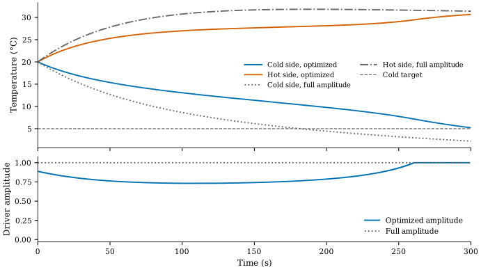
Figure 7:Cold and hot temperatures under the baseline plan, with a constant full-amplitude rollout for comparison. The lower panel shows their driver amplitudes. The target line and temperature traces show the tradeoff between energy use and final cold temperature.
The baseline plan drives relatively hard at first, eases off, then ramps to full amplitude near the deadline. Early driving uses the initially small temperature span, but it also warms the hot side and weakens later pumping. The fixed load adds the same total heat over every 300-second plan. Control timing still changes the temperature span and therefore the final cold temperature. Running at full amplitude throughout uses about and reaches ; its nonlinear cost is 149.886, versus 51.224 for the baseline local plan. The soft terminal cost need not favor the coldest possible final state.
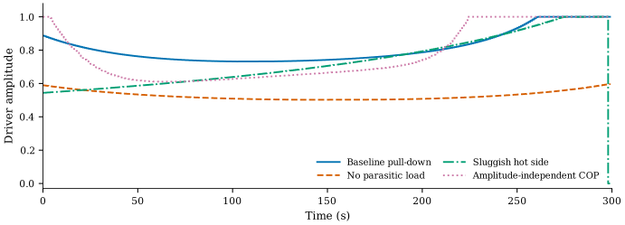
Figure 8:Final computed amplitude schedules for the baseline, no-load, sluggish-hot-side, and no-cubic-loss cases. The first three are iLQR plans; the no-cubic-loss plan is from DDP. Removing the cold-side load flattens the schedule, while changing the hot-side dynamics produces a long ramp.
Without the parasitic load, a nearly constant amplitude is economical. To see the tendency, temporarily hold the temperature span fixed and write . Heat pumped is then proportional to , while the cubic loss is proportional to , a convex function for . For a fixed total amount of pumping, Jensen’s inequality favors spreading through time. The actual schedule is not exactly constant because the span and hot-side temperature still respond to the controls. With and , the amplitude rises through most of the horizon, then turns off for the final two intervals. Both thermal storage and heat rejection changed in that experiment, so it does not isolate the effect of either parameter.
The DDP curvature term also has a direct physical interpretation here. For the continuous cold-side equation,
Increasing the temperature span weakens pumping, and this mixed derivative measures how that effect changes with amplitude. The solver differentiates the complete RK4 transition, whose Hessian also contains effects from the intermediate integration stages.
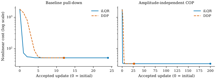
Figure 9:Actual nonlinear cost after each accepted update for iLQR and DDP in the baseline and no-cubic-loss cases. The vertical axis is logarithmic. The curves compare these local solves from the same initial control sequence, not a general ranking of the methods.
When , both pumping and work are quadratic in amplitude at a fixed temperature span. Their instantaneous ratio then no longer depends on amplitude, leaving weaker preferences among some schedules. In the recorded run, iLQR reaches its iteration limit while DDP satisfies the stopping test; both reach nearly the same final cost. For the sluggish hot side, DDP reaches a different, slightly lower-cost local plan than iLQR. Lowering the target to produces a plan saturated at throughout the fixed horizon, exercising the box-constrained backward step. These outcomes depend on the initial sequence. Starting the baseline from constant amplitudes 0.1 and 0.9 leads to other local plans, so neither result certifies a global minimum.
Exercises
Solution to Exercise 1
The last control is , and its minimized tail is . With , minimizing the remaining expression gives , followed by the same value for . Thus . As the terminal weight grows, the two controls tend to and the terminal state tends to .
Solution to Exercise 2
The local expansions are exact. Backward elimination therefore minimizes the original quadratic problem in perturbation coordinates, and recovers its solution. The affine simulator agrees exactly with the linearized perturbation dynamics. All transition Hessians vanish, so DDP produces the same correction. This is also a useful implementation test: compare the returned controls with a dense solve of the reduced quadratic objective.
Solution to Exercise 3
The Euler velocity update contains . The mixed derivative is therefore . DDP multiplies it by the component of and adds it to the corresponding state--control curvature entry. iLQR uses the first-order transition, whose second derivatives are zero within the local model. The actual experiment differentiates RK4 instead, so its mixed derivative includes the intermediate integration stages.
Solution to Exercise 4
Use make_problem(velocity_weight=0.) and keep every other choice fixed for
the first comparison. For the shorter experiment, set steps=80 in
BoatParameters and regenerate the initial controls. Removing the terminal
velocity term removes an explicit incentive to stop at the final time.
Running position and velocity costs can still lead to a slow arrival,
especially over the longer horizon, so failure is not inevitable. Measure
the final speed independently of position error and retain the same docking
tolerances for both objectives. A low-cost pass through the target is not
a successful stationary arrival.
Solution to Exercise 5
Fixing one coordinate at a bound changes the stationarity equation for the other coordinate through the off-diagonal entry of . Componentwise clipping does not solve that new equation. The face minimization does. If no nonlinear trial is accepted, the solver retains its previous controls and states and reports that it could not make progress; it must not replace them with an unaccepted trial or report convergence from rejection alone.
Solution to Exercise 6
With no load, cooling obtained early is not directly undone by a constant heat leak. If the temperature span were fixed, a given amount of cooling would fix the sum of . The cubic loss is proportional to , so Jensen’s inequality favors equal across time. The temperature span still evolves, which explains the modest variation in the computed schedule. With the load restored, the longer horizon admits lower amplitude over more intervals, but the leak adds heat throughout that extra time. In this model, the local solution starts near 0.59, reaches 0.89 by , and uses full amplitude in the final intervals. Its approximately of energy exceeds the shorter baseline’s use.
Computational Sources
The implementation separates the generic backward recursion from the physical models and artifact builders:
Run uv run python scripts/build_boat_docking_artifacts.py from the repository
root to reproduce the solves, figures, results table, and browser data. Normal
book builds read those artifacts. Tests independently check the derivatives,
the composed DDP curvature, the scalar calculation, and agreement between
backward elimination and a dense quadratic solve.
Run uv run python scripts/build_thermoacoustic_pulldown_artifacts.py to
regenerate the refrigerator results table, figures, diagnostics, and the
browser replay data.
Summary and Outlook
A feasible nonlinear rollout supplies the point around which dynamics and costs are approximated. Backward elimination of a local quadratic problem then supplies both a feedforward change and a state-dependent correction. iLQR repeats that calculation with linearized dynamics; DDP includes the second-order chain-rule terms from the transition. Nonlinear rollouts, regularization, and acceptance tests connect these local calculations to a decreasing sequence of actual trajectory costs. The refrigerator applies the same calculation to a bounded driver amplitude, with energy use and terminal temperature competing in the objective.
The docking and refrigerator experiments both use discrete transitions obtained by integrating ordinary differential equations. Continuous-time transcription and collocation develops other ways to represent continuous trajectories inside a finite optimization problem. Later, finite-horizon dynamic programming gives a broader interpretation of the quadratic tail: in the linear-quadratic case, the function produced by elimination is the optimal cost-to-go.
- Li, W., & Todorov, E. (2004). Iterative Linear Quadratic Regulator Design for Nonlinear Biological Movement Systems. Proceedings of the First International Conference on Informatics in Control, Automation and Robotics, 1, 222–229. https://roboti.us/lab/papers/LiICINCO04.pdf
- Tassa, Y., Mansard, N., & Todorov, E. (2014). Control-Limited Differential Dynamic Programming. IEEE International Conference on Robotics and Automation, 1168–1175. 10.1109/ICRA.2014.6907001
- Swift, G. W. (1988). Thermoacoustic engines. The Journal of the Acoustical Society of America, 84(4), 1145–1180. 10.1121/1.396617
- Swift, G. W. (2017). Thermoacoustics: A Unifying Perspective for Some Engines and Refrigerators (2nd ed.). Springer Cham. 10.1007/978-3-319-66933-5