MPC creates feedback by solving a new trajectory problem from each measured state. Can the decisions for an entire family of states be computed in advance instead? Dynamic programming decomposes a finite-horizon control problem into cost-to-go functions indexed by time and state.
The deterministic discrete-time optimal control problem provides the starting point. Stochastic successors will enter in the next chapter through conditional expectations.
Consider a typical DOCP of Bolza type:
Rather than considering only the total cost from the initial time to the final time, dynamic programming introduces the concept of cost from an arbitrary point in time to the end. This leads to the definition of the “cost-to-go” or “value function” :
This function represents the total cost incurred from stage onwards to the end of the time horizon, given that the system is initialized in state at stage . Suppose the problem has been solved from stage to the end, yielding the optimal cost-to-go for any state at stage . The question then becomes: how does this information inform the decision at stage ?
Given knowledge of the optimal behavior from onwards, the task reduces to determining the optimal action at stage . This control should minimize the sum of the immediate cost and the optimal future cost , where is the resulting state after applying action . Mathematically, this is expressed as:
This equation is known as Bellman’s equation, named after Richard Bellman, who formulated the principle of optimality:
An optimal policy has the property that whatever the previous state and decision, the remaining decisions must constitute an optimal policy with regard to the state resulting from the previous decision.
In other words, any sub-path of an optimal path, from any intermediate point to the end, must itself be optimal. This principle is the basis for the backward induction procedure which computes the optimal value function and provides closed-loop control capabilities without having to use an explicit NLP solver.
Dynamic programming can handle nonlinear systems and non-quadratic cost functions naturally. It provides a global optimal solution, when one exists, and can incorporate state and control constraints with relative ease. These advantages come from a change in what is being computed. Trajectory optimization takes the initial state as given and returns one sequence of states and controls, typically a local optimum. With state dimension and control dimension , the resulting nonlinear program has on the order of decision variables, so its size grows only linearly with the horizon and the dimension. Parametric optimization widened the question to a family of problems indexed by the initial state, but still answered it locally: sensitivity updates carry the solution of one instance to a nearby one, and learned controllers are fitted only on states sampled from the operating domain. Backward recursion asks for the optimal cost-to-go and the optimal decision from every state at every stage. The answer is a function on the whole state space rather than a vector of decision variables.
Representing such a function is what becomes expensive as the dimension of the state space increases, a difficulty Bellman termed the “curse of dimensionality.” If each of the state coordinates is discretized into levels, the table storing has entries, and each entry requires its own minimization over the controls. Computation and memory therefore grow exponentially with the state dimension, rendering direct application of dynamic programming intractable for high-dimensional problems. The curse is the price of asking for a solution everywhere. Trajectory optimization gives up the global, closed-loop answer to keep its cost polynomial in the dimension; dynamic programming obtains that answer and pays for it with exponential growth.
Fortunately, learning-based methods offer efficient tools to combat the curse of dimensionality on two fronts: by using function approximation (e.g., neural networks) to avoid explicit discretization, and by leveraging randomization through Monte Carlo methods inherent in the learning paradigm. Most of this course is dedicated to those ideas.
Backward Recursion
How does the terminal cost propagate backward into an optimal action and value for every earlier state?
The principle of optimality provides a methodology for solving optimal control problems. Beginning at the final time horizon and working backwards, at each stage the local optimization problem given by Bellman’s equation is solved. This process, termed backward recursion or backward induction, constructs the optimal value function stage by stage.
Upon completion of this backward pass, we now have access to the optimal control to take at any stage and in any state. Furthermore, we can simulate optimal trajectories from any initial state and applying the optimal policy at each stage to generate the optimal trajectory.
The proof uses a “cut-and-paste” argument. Any control sequence can be cut after its first step and its tail replaced by an optimal continuation without increasing its cost. Comparing first steps, each followed by its optimal continuation, then gives a sequence that no other sequence can beat. Figure 1 follows these two moves with concrete costs.
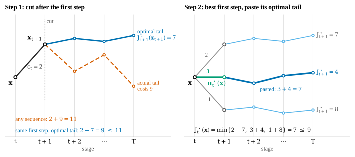
Figure 1:One inductive step of the proof of Theorem 1 with concrete costs. Step 1 (cut): an arbitrary sequence from costs . Keeping its first step and replacing its tail by the optimal tail from gives , so the sequence costs at least . Step 2 (paste): the top candidate is the first step of Step 1. Among the three first steps, each followed by its optimal tail, the middle one is cheapest, and its total is . The sequence of Step 1 costs at least this much (), and pasting the optimal tail to attains it.
Example: Seasonal Operation of a Hydroelectric Reservoir
On a northern river, most of the water arrives in a few weeks of spring, when the snowpack melts. This is the freshet. Electricity is worth the most in winter, when heating demand peaks. A reservoir behind a dam moves water from one season to the other. Each week the operator decides how much water to send through the turbines. Water released now is sold at this week’s price. Water kept in the reservoir can be sold later, and it also raises the water level, so every cubic metre released afterwards falls from a greater height and produces more energy. Keeping water has a risk as well. When the freshet reaches a full reservoir, the excess goes over the spillway and earns nothing.
The hydro cascade in the trajectory optimization chapter computed one plan from one initial state. An operator needs more than that. Inflows never follow the forecast exactly, so the reservoir is rarely at the level the plan assumed, and the operator needs a release for whatever level it is at. Dynamic programming provides this: one backward pass gives a release for every week and every storage level. Reservoir operators call the resulting curves rule curves, and dynamic programming has been used to compute them for decades Yeh, 1985.
Model. The stage is one week, with weeks starting in January. Volumes are measured in cubic hectometres ().
| Symbol | Meaning | Value |
|---|---|---|
| storage at the start of week (state) | ||
| water released through the turbines (control) | ||
| inflow forecast for week | 60 to 400 hm³/week | |
| electricity price in week | 30 to 90 $/MWh | |
| dead storage (below the intake) and capacity | 200 and 2000 hm³ | |
| ecological minimum flow and turbine capacity | 30 and 250 hm³/week | |
| head: height through which the water falls | 40 to 80 m | |
| energy per hm³ per metre of head | 2.45 MWh |
The inflows and prices are stylized curves, not measurements: a winter base flow of 100 m³/s, a freshet that peaks in mid-May at about four times the mean flow, an autumn rise from rain, and a price that is highest in early February and lowest in August. Water above capacity spills, so storage evolves as
Releasing with head produces megawatt-hours, where joules per cubic metre per metre, converted to MWh per hm³. The head grows with storage, which is what makes keeping water valuable beyond its later sale price. Water left at the end of the year is credited at $/MWh, so the terminal value is . Since the objective is a revenue to maximize rather than a cost, Bellman’s equation takes a maximum:
The bracket weighs the revenue earned by releasing this week against the revenue still obtainable from the storage that remains.
Code. The storage grid has a step of 10 hm³, and the inflows are rounded to
multiples of 10 hm³. Every successor is therefore a grid point,
and Algorithm 1 applies as stated:
is looked up, never interpolated. The next section removes this convenience.
The loop over states and actions of the algorithm is written with NumPy
broadcasting: x is a column of all storage levels and u a row of all
releases, so each line evaluates every (storage, release) pair at once.
import numpy as np

# Calendar: 52 weekly decisions; week 0 is the first week of January.
T = 52
weeks = np.arange(T)

# Inflow forecast w_t (hm³ per week): winter base flow, spring freshet, autumn rain.
w = 60 + 340 * np.exp(-((weeks - 19) / 3.5) ** 2) + 60 * np.exp(-((weeks - 43) / 4) ** 2)
w = 10 * np.round(w / 10)            # multiples of the grid step

# Price p_t ($/MWh): winter peak, summer trough.
p = 60 + 30 * np.cos(2 * np.pi * (weeks - 5) / 52)

# Reservoir and plant.
x_min, x_max = 200, 2000             # dead storage and capacity (hm³)
u_min, u_max = 30, 250               # ecological minimum and turbine capacity (hm³/week)
kappa = 2.45                         # MWh per hm³ per metre of head
p_T = 50                             # $/MWh credited to water left at the end of the year

def head(x):                         # metres of head; grows with storage
    return 40 + 40 * np.sqrt(x / x_max)

def terminal_value(x):
    return p_T * kappa * head(x) * (x - x_min)

dx = 10
X = np.arange(x_min, x_max + dx, dx)   # storage grid: 181 levels
U = np.arange(u_min, u_max + dx, dx)   # release grid: 23 levels

def index(x):                          # position of an on-grid storage level
    return np.round((x - x_min) / dx).astype(int)

J = np.zeros((T + 1, len(X)))
policy = np.zeros((T, len(X)))
J[T] = terminal_value(X)

for t in reversed(range(T)):
    x, u = X[:, None], U[None, :]                  # all (storage, release) pairs
    x_next = np.minimum(x + w[t] - u, x_max)       # water above capacity spills
    feasible = x + w[t] - u >= x_min               # cannot draw below dead storage
    value = p[t] * kappa * head(x) * u + J[t + 1][index(np.maximum(x_next, x_min))]
    value = np.where(feasible, value, -np.inf)
    J[t] = value.max(axis=1)
    policy[t] = U[value.argmax(axis=1)]

def simulate(x0):
    storage = [x0]
    for t in range(T):
        u = policy[t, index(storage[-1])]
        storage.append(min(storage[-1] + w[t] - u, x_max))
    return np.array(storage)

print(f"optimal revenue from x0 = 1100 hm³: {J[0, index(1100)] / 1e6:.1f} M$")
optimal revenue from x0 = 1100 hm³: 74.1 M$
The backward pass evaluates (week, storage, release) triples and takes a fraction of a second. Its output is not one trajectory but two tables, and , with one entry for every week and storage level.
Figure 2:Output of one backward pass. Left, the optimal release for every week and storage level, below the inflow forecast. Right, the water value , the revenue that one more hm³ in storage would add, below the price. White curves are the storage paths obtained by following the policy from five initial levels; after a few weeks they coincide.
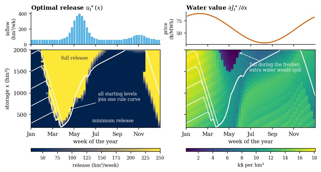
The left map is the policy. It has two regions: release at turbine capacity or release the ecological minimum, with a thin boundary between them. The white storage paths read the policy as an operator would. Whatever the level in January, the reservoir is drawn down to dead storage by late March, refilled by the freshet and then more slowly through the summer until it is full in mid-September, held full until late November, and drawn down at turbine capacity in December, when prices are high again. The initial storage affects only the first few weeks, because every path reaches the same rule curve before the freshet. A fuller reservoir in January simply means more water to sell during the winter drawdown.
The right map is the derivative of the value function with respect to storage, which hydro operators call the water value. It is lowest, close to zero, at full storage during the freshet: the reservoir cannot hold more, so an extra hm³ would spill and earn nothing. It is highest in winter at low storage, when every hm³ can be sold at the winter price and none is at risk of spilling.
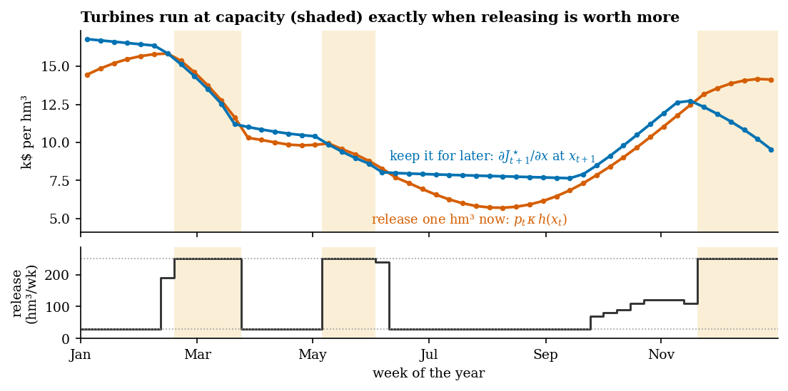
Why the policy is all or nothing. The release enters the bracket of Bellman’s equation twice: it earns per hm³ now, and it lowers next week’s storage, which costs per hm³. The derivative of the bracket with respect to is
Revenue now grows linearly in . When this difference is positive, releasing more increases the bracket, so the release goes to turbine capacity. When it is negative, the release falls to the minimum. The release lies strictly between the bounds only when the two terms are equal. The decision rule is therefore a price comparison: run the turbines when the price exceeds the value of the water in the reservoir, both expressed per hm³. In hydro-dominated power systems such as Norway’s, producers compute water values with dynamic programming and use them to set the prices at which they offer their energy.
Figure 3:The two terms of the derivative along the optimal path from hm³. The turbines run at capacity (shaded weeks) when the revenue from releasing one hm³ now (orange) exceeds the value of keeping it (blue), and at the ecological minimum when it is lower. From September to November the reservoir is full and any water kept would spill, so the release equals the inflow even though keeping water appears more valuable.
operating rule                      revenue (M$)  spill (hm3)
dynamic programming                         74.1            0
run of river (release = inflow)             66.8            0
full release when price > mean              63.4          900
The table above the figure compares the policy with two simpler operating rules over the same year. Running the river as it comes, releasing each week’s inflow, earns about 10% less because it sells most of the water during the freshet, when prices are low. Releasing fully whenever the price is above its annual mean earns even less and spills 900 hm³, because the rule ignores the storage level. It empties the reservoir by early February and has only the small winter inflow to sell for the rest of the high-price season. In May, when the price falls below its mean, it switches to the minimum release in the middle of the freshet. The reservoir is full by late June, and from July to November every hm³ above the minimum flow spills. Dynamic programming accounts for the price, the head and the remaining capacity at the same time, through one function of storage.
Explore the solution. The page below re-solves the same backward recursion in your browser whenever a parameter changes. Backward pass animates the recursion: the maps fill in from week 52 back to week 1, one column per Bellman update, and the panel beside the map shows the value function of the column being computed. Play the year then operates the reservoir forward from the chosen initial storage. The page compares the two terms of the derivative per MWh rather than per hm³: dividing both by turns the first into the price and the second into a water value in $/MWh.
Figure 4:The reservoir problem re-solved in the browser. The map shows the release, the water value or the value function over (week, storage); the side panel shows for the current week, whose slope is the water value. The strips compare the price with the water value along the simulated year and show inflow, release and spill.
Question. Set the price of water left at the end of the year to zero. What does the policy do in November and December? Is this what an operator who will still run the dam next year should do?
Answer
It empties the reservoir to dead storage by the end of December, because the model gives no value to water that remains after week 52. A real operator would start January with an empty reservoir and no water to sell during the high-price weeks. This end-of-horizon effect is an artifact of truncating the problem at one year. The terminal value stands in for the years that follow; the infinite-horizon formulations of later chapters remove the need to choose it.
Question. Starting from 1100 hm³, the policy keeps the minimum release through January, although the price is already above 80 $/MWh, and releases at full capacity from mid-February to mid-March. Why does it wait?
Answer
The reservoir must be nearly empty before the freshet starts in April, so the amount of water to sell before then is fixed. Two effects make it better to sell it late rather than early. The price keeps rising until early February. And water released later falls from a fuller reservoir: holding it keeps the head high, so every hm³ produces more energy. The turbines release at most 250 hm³ per week, about 190 hm³ net of the winter inflow, so emptying the reservoir takes about six weeks, and the policy starts the drawdown just early enough to finish before the freshet.
Question. Suppose the river had three such reservoirs in series, each discretized with the same 181 storage levels and 23 releases. How many (storage, release) combinations would one Bellman update have to evaluate at each week?
Answer
The state is the vector of the three storages, with grid points, and each has joint releases, so about evaluations per week instead of . This is the curse of dimensionality from the start of the chapter, and the reason the cascade was solved by trajectory optimization from one initial state.
Handling Continuous Spaces with Interpolation
When the next state falls between stored grid points, which interpolation rule supplies its continuation value without destroying the recursion?
In many real-world problems, such as the reservoir example, the state space is inherently continuous. Dynamic programming, however, is usually defined on discrete state spaces. To reconcile this, we approximate the value function on a finite grid of points and use interpolation to estimate its value elsewhere.
The reservoir example avoided this question by construction. Its inflows were rounded to multiples of the 10 hm³ grid step, so every successor landed exactly on a grid point. Measured inflows are not multiples of anything: a week with 63.7 hm³ of inflow and a 30 hm³ release sends a reservoir at 1000 hm³ to 1033.7 hm³, which lies between two grid points. The simplest response is to round the successor to the closest grid point and use the value stored there. This is nearest-neighbor interpolation, the zeroth-order case: the value function is treated as constant between grid points and equal to its value at the closest one.
While easy to implement, nearest-neighbor interpolation can introduce artifacts:
Decisions may change abruptly, even if the state only shifts slightly.
Precision is lost, especially in regimes where small variations matter.
The curse of dimensionality forces an impractically fine grid if many state variables are added.
To address these issues, we can use higher-order interpolation. Instead of taking the nearest neighbor, we estimate the value at off-grid points by leveraging multiple nearby values.
Backward Recursion with Interpolation
Suppose we have computed only at grid points . To evaluate Bellman’s equation at an arbitrary , we interpolate. Formally, let be the interpolation operator that extends the value function from to the continuous space. Then:
For instance, in one dimension, linear interpolation gives:
where and are the nearest grid points bracketing . Linear interpolation is often sufficient, but higher-order methods (cubic splines, radial basis functions) can yield smoother and more accurate estimates. The choice of interpolation scheme and grid layout both affect accuracy and efficiency. A finer grid improves resolution but increases computational cost, motivating strategies like adaptive grid refinement or replacing interpolation altogether with parametric function approximation which we are going to see later in this book.
In higher-dimensional spaces, naive interpolation becomes prohibitively expensive due to the curse of dimensionality. Several approaches such as tensorized multilinear interpolation, radial basis functions, and machine learning models address this challenge by extending a common principle: they approximate the value function at unobserved points using information from a finite set of evaluations. However, as dimensionality continues to grow, even tensor methods face scalability limits, which is why flexible parametric models like neural networks have become essential tools for high-dimensional function approximation.
Example: Reservoir Operation with Unrounded Inflows
We return to the reservoir with the inflow forecast left unrounded, so that
successors fall between grid points, and solve it on a coarse grid of 19
storage levels spaced 100 hm³ apart. Two versions of
Algorithm 2 differ only in the interpolation rule
passed to them: nearest neighbor or linear (np.interp). A reference solution
uses linear interpolation on a grid twenty times finer. Each value function is
then used the way an operator would use it: the reservoir is simulated with the
exact, unrounded dynamics, and each week’s release is chosen by one Bellman
step with the interpolated .
# Unrounded inflows: successors now fall between grid points.
w_raw = 60 + 340 * np.exp(-((weeks - 19) / 3.5) ** 2) + 60 * np.exp(-((weeks - 43) / 4) ** 2)
U_fine = np.linspace(u_min, u_max, 45)

def nearest(x_query, grid, values):
    step = grid[1] - grid[0]
    i = np.clip(np.round((x_query - grid[0]) / step).astype(int), 0, len(grid) - 1)
    return values[i]

def linear(x_query, grid, values):
    return np.interp(x_query, grid, values)

def backward_recursion(grid, interpolate):
    J = np.zeros((T + 1, len(grid)))
    J[T] = terminal_value(grid)
    for t in reversed(range(T)):
        x, u = grid[:, None], U_fine[None, :]
        x_next = np.clip(x + w_raw[t] - u, x_min, x_max)
        value = p[t] * kappa * head(x) * u + interpolate(x_next, grid, J[t + 1])
        J[t] = np.where(x + w_raw[t] - u >= x_min, value, -np.inf).max(axis=1)
    return J

def operate(grid, J, interpolate, x0):
    """Simulate the true dynamics, choosing each release by one Bellman step."""
    storage, revenue = [x0], 0.0
    for t in range(T):
        x = storage[-1]
        x_next = np.clip(x + w_raw[t] - U_fine, x_min, x_max)
        value = p[t] * kappa * head(x) * U_fine + interpolate(x_next, grid, J[t + 1])
        u = U_fine[np.argmax(np.where(x + w_raw[t] - U_fine >= x_min, value, -np.inf))]
        revenue += p[t] * kappa * head(x) * u
        storage.append(min(x + w_raw[t] - u, x_max))
    return np.array(storage), revenue + terminal_value(storage[-1])

coarse = np.arange(x_min, x_max + 100, 100)   # 19 levels
fine = np.arange(x_min, x_max + 5, 5)         # 361 levels
schemes = {
    "fine grid, linear (reference)": (fine, linear),
    "coarse grid, nearest neighbor": (coarse, nearest),
    "coarse grid, linear": (coarse, linear),
}
outcomes = {}
for name, (grid, interpolate) in schemes.items():
    J_scheme = backward_recursion(grid, interpolate)
    storage, revenue = operate(grid, J_scheme, interpolate, 1100)
    outcomes[name] = (grid, J_scheme[0], storage)
    print(f"{name:<32} predicted {linear(1100, grid, J_scheme[0]) / 1e6:6.2f} M$"
          f"   realized {revenue / 1e6:6.2f} M$")
fine grid, linear (reference) predicted 74.16 M$ realized 74.17 M$
coarse grid, nearest neighbor predicted 98.46 M$ realized 71.06 M$
coarse grid, linear predicted 74.02 M$ realized 74.15 M$
Figure 5:Coarse-grid solutions of the reservoir problem with unrounded inflows. Left, the value function at the start of the year. Nearest-neighbor rounding (dashed) predicts far more revenue than the reference; linear interpolation on the same 19 points (blue) lies on the reference (grey). Right, storage when each value function is used to operate the reservoir from 1100 hm³. The nearest-neighbor policy never fills the reservoir in summer.
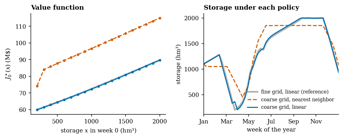
Linear interpolation on 19 points predicts a revenue within 0.2% of the 361-point reference and realizes one within 0.03%. Nearest-neighbor rounding on the same grid fails in two ways, and both come from the size of a typical weekly change. In summer the reservoir gains about 30 hm³ per week at the minimum release, less than half the grid step, so the rounded successor equals the current grid point. Storing water appears to gain nothing, so the policy releases the summer inflow at summer prices instead of keeping it for winter, and the reservoir never fills. The value function is also too optimistic, by about a third. The maximization over releases chooses, among actions whose successors round to different grid points, the ones whose rounding adds water that does not exist. Errors that would average out under a fixed policy accumulate under optimization, because the maximum selects them. Linear interpolation keeps the fractional part of every step, so small changes accumulate correctly over the year.
Linear Quadratic Regulator via Dynamic Programming
What form do the value function and feedback law take when the dynamics are linear and every cost is quadratic?
The successive-approximation chapter obtained a quadratic tail by eliminating controls backward. In the linear-quadratic case, that tail is the optimal cost-to-go. Bellman’s equation therefore gives another derivation of the same Riccati recursion.
Linear dynamics and quadratic costs give a backward recursion that can be solved in closed form. The value function remains quadratic at every stage, and the optimal policy is a linear feedback law. No state grid, interpolation scheme, or general function approximator is needed. The recursion tracks a finite sequence of matrices.
Consider a discrete-time linear system:
where is the state and is the control input. The matrices and describe the system dynamics at time .
The cost function to be minimized is quadratic:
where (positive semidefinite), , and (positive definite) are symmetric matrices of appropriate dimensions. The positive definiteness of ensures the minimization problem is well-posed.
A quadratic terminal cost implies a quadratic value function at every earlier stage. Suppose the optimal cost-to-go at stage has the form
for some positive semidefinite matrix . At the terminal time, this is true by definition: .
Backward induction verifies the hypothesis. Assume . Bellman’s equation at stage is
Substituting the dynamics and the quadratic form for :
Expanding the last term:
The expression inside the minimization becomes:
Collecting terms involving :
This is a quadratic function of . To find the minimizer, we take the gradient with respect to and set it to zero:
Since is positive definite (both and are positive semidefinite with strictly positive), we can solve for the optimal control:
Define the gain matrix:
so that . This is a linear feedback policy: the optimal control is simply a linear function of the current state.
Substituting back into the cost-to-go expression and simplifying (by completing the square), we obtain:
where satisfies the discrete-time Riccati equation:
The resulting backward recursion is:
Local Stabilization of the Cart-Pole
The cart-pole in the trajectory-optimization chapter started from the downward configuration and required a large nonlinear maneuver to reach the top. Once it is near the upright equilibrium, a smaller problem remains: reject local deviations by moving the cart in response to the measured state. The nonlinear state and input are the same as before,
with at upright. Linearizing the discrete RK4 update at gives
The experiment uses s, , and . For this time-invariant infinite-horizon case, the Riccati recursion converges to a fixed matrix that satisfies the discrete algebraic Riccati equation. The corresponding policy is .
The unconstrained linear closed loop is asymptotically stable when every eigenvalue of lies inside the unit disk. The physical implementation adds two constraints that are absent from that eigenvalue calculation: acceleration is clipped to , and the cart must remain inside a 2.4 m rail. Three deterministic nonlinear rollouts distinguish the claims supported by the linearization:
An uncontrolled pole begins from upright.
The LQR controller begins from the same displacement.
The same controller begins from upright with the same actuator and rail limits.
Figure 6:The discrete linear closed loop is stable, and the nonlinear controller recovers from a 5 degree perturbation. Without control, the same initial displacement grows. From 45 degrees, the commanded acceleration saturates and the cart reaches its rail limit, so the local controller does not complete the recovery. All curves use the same nonlinear plant; only the initial state and controller differ.
closed-loop spectral radius: 0.9824
uncontrolled, 5 deg    not stabilized final angle= -71.71 deg max |x|= 0.00 m max |u|= 0.0 m/s^2
LQR, 5 deg             stabilized     final angle=  -0.00 deg max |x|= 0.15 m max |u|= 4.0 m/s^2
LQR, 45 deg            rail limit     final angle= 146.84 deg max |x|= 2.40 m max |u|= 8.0 m/s^2
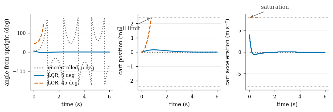
The closed-loop eigenvalues certify asymptotic stability of the unconstrained linearized model, not every trajectory of the nonlinear constrained plant. The rollout remains in a region where the linear approximation supplies useful actions. The rollout immediately asks for more acceleration than the actuator can provide, then exhausts the available rail. Increasing the entries of cannot remove those physical limits.
Figure 7:Nonlinear validation of the local LQR controller. The left panel shows the uncontrolled fall from 5 degrees, the center panel shows recovery from the same state, and the right panel shows the 45 degree rollout ending at the rail limit. Python generates each frame from the recorded trajectories.
Balancing a pen on a finger motivates the action channel because the finger stabilizes the object by moving its base. The cart-pole model replaces the contact by a planar frictionless hinge. A real pen can slip, detach, flex, and rotate out of the plane, while sensing and hand motion introduce delays. The calculation establishes local stabilization for the stated rigid-body model; the classroom demonstration shares its instability and feedback mechanism, not all of its equations.
Inspect the linearization and LQR design
1 2 3 4 5 6 7 8 9 10 11 12 13 14 15 16 17 18 19 20 21 22 23 24 25 26 27 28 29 30 31 32 33 34 35 36 37 38 39 40 41 42 43 44 45 46 47 48 49 50 51 52 53 54 55def linearize_upright( parameters: CartPoleParameters = CartPoleParameters(), *, step_size: float = 0.02, epsilon: float = 1e-6, ) -> tuple[np.ndarray, np.ndarray]: """Linearize the exact discrete RK4 update at the upright equilibrium.""" equilibrium = np.zeros(4) state_matrix = np.empty((4, 4), dtype=float) for column in range(4): perturbation = np.zeros(4) perturbation[column] = epsilon state_matrix[:, column] = ( rk4_step(equilibrium + perturbation, 0.0, parameters, step_size) - rk4_step(equilibrium - perturbation, 0.0, parameters, step_size) ) / (2.0 * epsilon) input_matrix = ( rk4_step(equilibrium, epsilon, parameters, step_size) - rk4_step(equilibrium, -epsilon, parameters, step_size) )[:, None] / (2.0 * epsilon) return state_matrix, input_matrix def design_lqr( parameters: CartPoleParameters = CartPoleParameters(), *, step_size: float = 0.02, ) -> LQRDesign: """Solve the discrete algebraic Riccati equation at the upright state.""" state_matrix, input_matrix = linearize_upright(parameters, step_size=step_size) cost_matrix = np.diag([2.0, 0.2, 80.0, 3.0]) control_cost = np.array([[0.15]]) riccati_matrix = solve_discrete_are( state_matrix, input_matrix, cost_matrix, control_cost, ) gain = np.linalg.solve( control_cost + input_matrix.T @ riccati_matrix @ input_matrix, input_matrix.T @ riccati_matrix @ state_matrix, ) eigenvalues = np.linalg.eigvals(state_matrix - input_matrix @ gain) return LQRDesign( state_matrix, input_matrix, cost_matrix, control_cost, riccati_matrix, gain, eigenvalues, )
Download the shared nonlinear cart-pole and LQR source.
Summary and Outlook
Backward recursion replaces one trajectory optimization with a sequence of state-indexed subproblems. Interpolation extends the recursion beyond a finite state grid, and the linear-quadratic case reduces the value function to a Riccati recursion and the policy to linear state feedback.
These recursions still assign one successor to each state and action. How do the value and policy change when a decision must account for a distribution of possible successors? Stochastic dynamic programming replaces the deterministic continuation value by a conditional expectation.
- Yeh, W. W.-G. (1985). Reservoir Management and Operations Models: A State-of-the-Art Review. Water Resources Research, 21(12), 1797–1818.