The preceding chapters formulated deterministic trajectory optimization as a nonlinear program. Shooting and collocation turn the dynamics, costs, and constraints into a finite-dimensional problem that we can solve with an NLP solver. Gradient-based methods are effective when accurate derivatives are available. How can we improve a trajectory when we can simulate the system and evaluate its cost, but differentiating through that computation is difficult or expensive?
Model predictive path integral control (MPPI) uses sampling to construct an update. It draws candidate control sequences, simulates their trajectories, and forms a weighted average that favors lower-cost outcomes. This requires no derivatives of the dynamics or cost, and the candidate rollouts can run in parallel. The derivation begins with a distribution over control sequences: costs determine which sequences receive more probability, and fitting a Gaussian to that distribution gives the weighted-average update. This construction applies even to a deterministic simulator. An aircraft example extends the calculation to uncertain winds by estimating each candidate flight’s expected cost before assigning its weight. A reactor example applies the same update to temperature and composition fields governed by a partial differential equation, first planning with the equation itself and then with a learned surrogate. Executing the first action and planning again from the next observation connects these computations to the following chapter on receding-horizon control.
Learning Goals
After working through the examples and exercises, you should be able to:
Calculate an MPPI update, including the correction for sampling around a nonzero nominal control sequence.
Derive exponential weighting from a KL-regularized objective and obtain the control update by fitting a Gaussian mean.
Distinguish samples used to explore controls from samples used to estimate a candidate’s expected cost under physical disturbances.
Assess a sampled plan using feasibility checks, weight concentration, and comparisons under shared disturbances.
Execute the first action of a sampled plan and update the remaining plan from new observations.
Reduce a field-control problem to a few bounded sampling parameters, and validate each sampled update in the full simulation before it replaces a feasible plan.
Prerequisites
The algorithm uses the single-shooting rollout and the finite-horizon optimal-control formulation. The sampling derivation requires Gaussian distributions and expectations; KL divergence and importance sampling are developed here. The aircraft example uses conditional disturbance models from Stochastic Dynamics and Partial Observation. The reactor example states the finite-volume model it uses and assumes no background in partial differential equations.
Improving a Control Sequence by Sampling
We already know how to evaluate a control sequence: simulate the system and compute the resulting cost. How can we improve that sequence? Instead of computing a gradient, we try many random variations, evaluate each one, and form a weighted average that gives more influence to the lower-cost candidates. That average becomes our next control sequence.
If the system has control components, then contains the inputs applied together at time step . The current plan collects these vectors over all steps. Thus is one step’s control vector, while is the complete sequence, with entries when stacked into one vector.
Draw Gaussian perturbation sequences and simulate each candidate . After assigning normalized weights to the resulting trajectories, form the new control sequence
The same trajectory weight multiplies every action in its sequence. How should those weights depend on the costs? Giving every candidate the same weight, , would ignore the rollout results. Because the perturbations have mean zero, this update would return on average, regardless of which candidates performed well. At the other extreme, assigning weight one to the lowest-cost candidate and zero to the others would select a single sequence. A candidate with a nearly identical cost would have no influence, and a small change in which candidate ranks first could switch the entire update.
MPPI allows several low-cost candidates to contribute, with their influence decreasing smoothly as cost increases. Consider first the initial sequence . The candidate sequences are then the zero-mean Gaussian perturbations themselves. This Gaussian is the reference distribution: it remains fixed even when later updates move the sampling mean away from zero. Let be the accumulated state cost along rollout , including its terminal cost. MPPI assigns it the positive score and divides by the sum of all scores:
This is the softmax of the negative costs, with temperature . The minus sign makes lower costs receive larger scores, and the denominator makes the weights sum to one. The parameter has the same units as cost, so is dimensionless. To see how it sets the strength of the preference, compare two candidates. Their common denominator cancels:
If rollout costs more than rollout , it receives half as much weight. Thus cost differences, rather than the arbitrary zero of the cost scale, determine relative influence. For a fixed batch, small makes even modest cost differences strongly affect the weights; large makes them less consequential. As , the weights concentrate on the lowest-cost candidate, or split equally among tied minima. As , they approach . These are the two alternatives above, now connected by a continuous weighting rule.
The curves in Figure 1 show this dependence on cost and temperature. Each curve compares a rollout’s weight with the weight of the best candidate in the same batch.
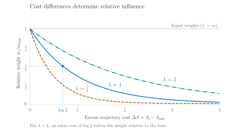
Figure 1:Smaller temperatures reduce the influence of higher-cost trajectories more sharply. With , the horizontal axis is the excess cost , and the vertical axis is the ratio . Costs and temperatures use the same arbitrary cost unit. The marked point shows that halves the relative weight when . The dotted horizontal line is the equal-weight limit as . A ratio of one at does not mean that the best rollout receives all the normalized weight: the actual still sum to one across the batch.
The Gaussian reference already favors small controls. Its contribution to control effort will appear explicitly in the distributional objective below; includes only state and terminal costs. The displayed weights apply when sampling from this reference, with . Sampling around a nonzero plan changes how often each candidate is drawn and requires a corresponding correction to its weight.
The computational attraction is that each rollout and cost evaluation can run independently, making large batches suitable for GPU execution Williams et al., 2017. This parallelism does not guarantee that a modest number of samples will find low-cost control sequences: long horizons, many control variables, and narrow feasible regions can make the search difficult. We will check both sampling quality and feasibility when using the update in the aircraft and reactor examples.
So far, exponential weighting is a rule for combining a batch of trials. To justify the rule, we need an objective whose solution gives those weights, and a reason to use their average as the next plan. Both follow by treating the candidate sequences as samples from a distribution and optimizing that distribution before fitting a new control sequence to it.
From Trajectory Weights to MPPI
Which optimization problem gives the exponential weights and their weighted-average update? A distribution over control sequences lets us balance low trajectory cost against a preference for small inputs. The resulting distribution need not have a simple form, but fitting a Gaussian to it produces a mean that can serve as the next plan. Sampling then estimates this mean. Throughout this derivation, randomness comes from the search over controls; the simulator itself can be deterministic.
Reference and sampling distributions
For a general rollout, write , where is the candidate control vector at step . Collect these vectors into the complete candidate sequence , with the same structure as the nominal sequence . The initial state is fixed, so each input sequence determines a simulated state sequence. Define the state and terminal cost of a rollout by
Each is the cost for one interval; if it comes from a continuous running cost, its discretization includes the interval length.
In the earlier optimal-control formulation, a stage cost could penalize both the state and the control effort. Here contains only the state cost; the inputs still affect through the simulated states. Control effort will be accounted for separately by a KL-divergence penalty between the input distribution and a reference distribution.
Choose a Gaussian reference distribution centered at zero to express a preference for small inputs. As derived below, this choice makes the KL penalty a quadratic cost on the magnitude of the nominal controls; the penalty vanishes when the nominal sequence is zero. Use a separate Gaussian sampling distribution over complete input sequences, centered at the current plan . At each step , the candidate control has mean under and mean under . Both use the same positive-definite covariance for the control components at a single step. Assuming independence across time gives the joint densities over the complete sequence:
Centering the reference at zero is a modeling choice. A Gaussian reference could instead be centered on a prescribed baseline sequence; the KL penalty would then charge for squared deviations of the nominal controls from that baseline. In either case, the state and terminal costs can favor controls away from the reference mean when their benefits justify the effort.
The reference remains fixed during a planning update. The sampling mean is the entire nominal sequence . This mean is taken over repeated candidate draws, with a separate mean control vector for each time step. Changing moves the center of the candidate controls at step . Initializing means setting every , so the sampling and reference distributions initially coincide. Later updates can change the nominal controls at each step, moving the samples toward a new plan while the reference stays centered at zero. The sampler can therefore change where it searches without changing the reference that defines the objective.
Exponentially weighting the reference
Sampling from the reference determines how often different input sequences appear in a batch. Assigning a cost weight to each draw then changes how much that occurrence contributes to the weighted average. The total weight assigned to a sequence depends on both its sampling frequency and its weight per occurrence, which is why these two factors multiply.
For example, first consider a reference with only two possible input sequences, and , selected with probabilities and . Suppose their costs are and , so each draw of receives score and each draw of receives score 1. Their reference probabilities multiplied by these scores are
Dividing by the sum, , gives probability to each sequence. The reference samples three times as often, but each occurrence receives one third of the weight, so the two effects cancel.
For continuous inputs, the same operation multiplies the reference density by the score at each sequence , then divides by the integral of that product:
The score is not itself a probability density, and the product does not define a joint distribution of two random variables. Both factors concern the same input sequence: specifies its density before costs are considered, and the score adjusts that density according to its cost. The normalizing constant makes the resulting density integrate to one.
Assume is measurable and bounded below and . The normalized result is a Gibbs distribution: two trajectories with equal reference density and cost difference have density ratio . The parameter has the units of cost and controls how strongly those costs affect the ratio.
The opening batch weights contain only the scores because drawing from already accounts for the reference probabilities. Multiplication by appears when we describe the distribution represented by those weighted samples. This explains how weighting changes a distribution; the particular choice of an exponential score is justified by the objective combining expected cost and KL divergence below.
The objective defined by the weights
The exponential weights solve an optimization problem over distributions of input sequences. We seek a distribution that reduces expected state and terminal cost while paying a penalty for departing from . Measure that departure with the Kullback--Leibler divergence. For densities , it is
This divergence is nonnegative and equals zero only when the two distributions agree. For it to be finite, must put no probability where has zero density, a condition called absolute continuity. With setting the cost of departure from the reference, the first optimization problem is
Here ranges over distributions on complete input sequences for which both terms are finite; it is not restricted to a Gaussian family.
Recall that is the distribution obtained by multiplying the reference density by the exponential cost score and normalizing. Its density is . To verify that this distribution solves the optimization problem, we can express the difference between and its minimum as a nonnegative divergence. Substituting this density into the logarithm gives
Taking the expectation under recovers the two terms in :
Rearranging isolates the objective:
The quantity is fixed by , , and , so the term does not depend on . Choosing makes the remaining term, , equal to zero. Every other distribution gives a positive divergence and hence a larger objective value. This proves that , with minimum value .
The exponential cost weight is contained in the definition of ; it is no longer explicit in the KL identity because we took logarithms. Writing out the density of the minimizing distribution gives
Multiplying the reference density by the indicated factor and normalizing by is the exponential weighting introduced above. The bound on proves that the distribution constructed this way solves (9).
For a Gaussian with the same covariance as the reference, the KL penalty is a quadratic function of its mean controls:
For example, choose , where is the interval length and specifies how costly each input direction is. Then this penalty is , the discretization of the control-effort integral for controls held constant on each interval. Thus, within this Gaussian family, departing from the zero-mean reference incurs a quadratic cost on the nominal controls. This accounts for control effort without adding it to . Changing with fixed changes this penalty as well as the concentration of the weights.
The solution assigns probabilities to complete input sequences. A controller still needs a nominal sequence to store and execute. We obtain that sequence by approximating with a Gaussian whose mean can be stored as a plan.
Fitting a Gaussian mean
The density is generally neither Gaussian nor independent across time. To approximate this distribution, consider the same Gaussian family as our sampler, with a candidate mean sequence :
Only the mean sequence is adjustable; the covariance at each step remains fixed. The second optimization problem chooses the Gaussian that minimizes its divergence from in the following direction:
Here is fixed, and the variable is a finite-dimensional mean sequence . Expanding this objective separates the two log densities:
The first expectation does not depend on . In the second, the Gaussian normalization also stays fixed because is fixed. Substituting the Gaussian log density therefore gives
The constant collects the terms in the divergence that do not depend on . Minimizing the divergence is thus equivalent to minimizing the expected squared distance from the candidate mean to an input sequence drawn from , with distances measured by . Assuming finite second moments, differentiation gives
Setting this gradient to zero yields the unique minimizer, since is positive definite:
With an exact solution of (16), the updated Gaussian would have the same mean as . The equation above identifies that mean as the quantity we need to compute; it does not yet provide a way to evaluate it. We know the density of up to its normalizing constant: for any candidate sequence , a rollout gives , so we can evaluate . In general, however, calculating or requires high-dimensional integration, and we do not have a direct sampler for .
Importance sampling in Correcting for where the samples were drawn will estimate this mean from candidates drawn from the Gaussian , which we can sample. The normalized weights will account for the difference between the two distributions without requiring the value of . Thus the computed update will only approximate the mean of ; the equality above describes the exact target of the calculation. The quadratic example below first provides a case where this target can be calculated analytically.
Even if its mean were computed exactly, the Gaussian would retain covariance at each step. It can therefore lose features of : if low-cost sequences form separate groups, their average can lie between those groups.
The first problem, (9), chooses an entire distribution by minimizing . The second, (16), holds its solution fixed and chooses a Gaussian mean by minimizing . If we instead restricted the first problem to Gaussians, the identity above would give
The order of the distributions in this divergence is reversed relative to (16). KL divergence is not symmetric, so these two choices of Gaussian mean need not agree Williams et al., 2017.
A one-step quadratic check
For a scalar system with and target 1, take with , , and . The dynamics are deterministic: different endpoints result from trying different inputs. Multiplying the reference density by and completing the square gives
Thus the first optimization problem has solution . Weighting has shifted the reference toward the target and reduced its variance. The second problem keeps the variance at its chosen value of one and adjusts only the Gaussian mean:
The resulting approximation is . It has the correct mean but is broader than . Figure Figure 2 shows both optimization steps for .
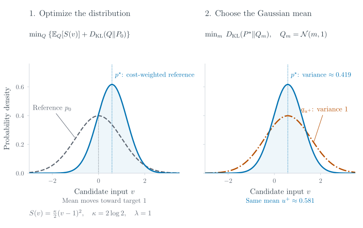
Figure 2:The two MPPI optimization problems change different properties of the input distribution. For the scalar rollout , target 1, cost , , and , the reference is . Left: minimizing expected cost plus gives the blue solid density , with mean and variance . The gray dashed curve is the reference. Right: minimizing over gives the orange dash-dotted density , with the same mean as and variance one. The vertical dotted lines mark the means. Both panels show analytic densities, without sampling error.
In this quadratic example, also minimizes the deterministic objective : setting its derivative to zero gives . This agreement checks the update in the example; taking the mean of need not minimize the deterministic cost for a general rollout.
To check the finite-sample calculation, set and start from . Suppose three draws from the reference, rounded for this calculation, are . Evaluating their costs gives
| Candidate input | Endpoint | Cost | Unnormalized weight | Normalized weight |
|---|---|---|---|---|
| -1 | -1 | |||
| 0 | 0 | |||
| 1 | 1 | 0 | 1 |
The weighted average is
This three-sample estimate, 0.6, is close to the exact mean . All three candidates contribute; the update does not simply select the best sampled input, 1. Sampling around the updated plan will produce a different mix of candidates, so preserving the same target mean requires adjusting their weights.
Correcting for where the samples were drawn
The mean is the exact solution of the Gaussian approximation problem. To estimate it for a general rollout, we have two available operations: draw a sequence from , and evaluate its cost . We can use these operations without a direct sampler for or an analytic value for its normalizing constant .
Substituting the definition of into the desired expectation and writing as its defining integral gives
Both integrals involve the unnormalized density that we can evaluate. Multiplying and dividing their integrands by expresses them as expectations under the distribution we can sample:
This change of sampling distribution is importance sampling. A batch from can estimate both expectations, using the score for each candidate. Dividing by the sum of these scores normalizes the sample weights, so we do not need to know .
For example, moving a scalar proposal to a positive mean makes positive inputs more common even if the target distribution has not changed. Weighting only by state cost would mistake that extra sampling frequency for additional target probability. The factor removes it. Since both Gaussians have full support, every trajectory with positive target density remains accessible. Writing and expanding their quadratic exponents gives
The last quadratic term is identical across samples and cancels from the normalized weights. Consequently each sampled sequence receives the corrected cost
A stable finite-sample update
The ratio of expectations above is exact. To compute an approximate update, replace both expectations by averages over independent samples from . For numerical stability, subtract before exponentiation. This common subtraction leaves normalized weights unchanged and avoids overflow:
The same full-trajectory weight updates every time slot. This ratio of sample averages is a self-normalized importance-sampling estimator. It is generally biased for finite and converges to the target mean when the relevant weighted moments are integrable. Further iterations move the proposal toward useful trajectories; with exact expectations, the target mean would already be independent of the proposal.
A quadratic rollout makes the effect of this correction explicit. Take , , , , and terminal cost . With and , the exact target mean is 0.8 at every time step. Sampling around and omitting the correction instead estimates 0.88, even with arbitrarily many samples. Exercise Exercise 2 derives both limits. Moving the proposal should change the accuracy of the estimate, not the mean being estimated.
Receding-horizon execution
The update gives a sequence of actions for a particular initial state. Model error or physical disturbances can make the next observed state differ from the rollout prediction. Continuing with the stored sequence would ignore that discrepancy. Instead, apply only the first action and use the newly observed state as the initial condition for another planning problem. MPPI repeats the trajectory computation from that condition, as in the sampling controllers of Williams et al. (2017).
This version assumes unrestricted Gaussian inputs and finite rollout costs. Nonconvex state constraints need additional treatment: even an average of inputs from feasible trajectories can generate an infeasible trajectory. Clipping samples also changes their density, so the displayed Gaussian likelihood ratio does not apply unchanged to the clipped variables. A chosen exploration covariance different from the reference covariance requires the full corresponding density ratio.
The rollouts can be simulated in parallel. Their effectiveness still depends on overlap between proposal and target. The quantity summarizes weight concentration: it is for equal weights and approaches one when a single rollout dominates. It diagnoses sampling concentration, rather than certifying optimality or constraint satisfaction. A finite-sample update can increase the rollout cost, particularly when only a few samples carry most of the weight. Concentrated weights suggest increasing the sample count or improving overlap between proposal and target. Increasing with a fixed reference weakens state-cost weighting, but also changes the optimization objective. Altering the proposal covariance alone requires the corresponding likelihood correction. Receding-horizon execution supplies feedback through repeated observations; the stored sequence itself is open loop.
Connection to diffusion-based planning
The distribution over low-cost plans also connects this computation to modern diffusion-based trajectory optimization. In model-based diffusion, the objective defines a target density through an exponential cost weight. Gaussian perturbations and cost-weighted averages then provide estimates used to refine trajectories through a sequence of noise levels Pan et al., 2024. MPPI’s weighted mean provides a useful starting point for understanding that construction. The MPPI update here uses a fixed sampling covariance and does not train a denoising network or run a diffusion noise schedule. In both algorithms, random perturbations can serve only to explore controls. Physical disturbances introduce a separate source of variation: a single candidate plan can produce different costs under different disturbance realizations. The aircraft example uses several simulated winds to estimate the cost assigned to each candidate.
Aircraft Planning Under Uncertain Winds
Consider an Airbus A320 flying from Montréal–Trudeau (CYUL) to Toronto–Pearson (CYYZ). The task is to choose climb, cruise, descent, and flight duration to use little fuel while arriving within 1 km horizontally and 30 m vertically of the destination. A favorable wind at one altitude may justify climbing, but its later evolution is uncertain. How can the sampled-control update account for these different possible outcomes when comparing candidate flights?
The method from From Trajectory Weights to MPPI can optimize an estimated expected cost from a simulator. It requires separate samples for candidate controls and for future winds: several winds must be evaluated before a candidate is assigned its cost weight. The following model makes those two random quantities explicit.
The airborne model and its wind state
In the OpenAP A320 point-mass model Sun, 2022, the state is : east and north position in a local map, altitude in meters, mass in kilograms, and elapsed time in seconds. Here denotes altitude; numerical time steps will be given in seconds. Controls are Mach number , vertical speed in meters per second, and heading in radians clockwise from north. If is true airspeed and , the model is
The horizontal equations separate air-relative motion from wind-driven
displacement: is the fixed mean wind field and is a gust.
Fuel flow reduces mass as the aircraft flies. The heading
convention and flight-path-angle approximation reproduce OpenAP.top’s
point-mass equations. Conversions to knots, feet, and feet per
minute occur only when calling OpenAP interfaces that require them. The
numerical derivatives are tested against OpenAP.top’s original symbolic
model at climb, cruise, and descent states. Optimization itself uses forward
simulation and Gaussian sampling.
The reference flight covers the complete airborne leg, with the following initial and nominal conditions:
| Quantity | Value |
|---|---|
| Initial mass | of maximum takeoff mass |
| Departure and arrival altitude | 100 ft |
| Nominal cruise altitude | 7000 m |
| Nominal duration | 3600 s |
Taxi, runway operations, and traffic are outside this model. Mach number,
vertical speed, heading, altitude, mass, and the geographic flight corridor have
explicit bounds. Thrust, lift, and excess-energy inequalities reproduce the
approximate OpenAP.top envelope checks. Adjacent command changes are also
checked against limits of 0.2 Mach, 500 ft/min in vertical speed, and
15 degrees in heading. These are constraints of the teaching model.
The mean field is the committed ERA5 pressure-level snapshot for June 1, 2023, at 12:00 UTC Copernicus Climate Change Service (C3S), 2018. Preprocessing converts the original GRIB values once to a numerical array. The simulator interpolates in pressure, latitude, and longitude, using ISA pressure at the aircraft’s altitude. Outside the snapshot’s pressure range of 200–925 hPa, it holds the boundary value; in particular, winds near the ground use the lowest available pressure level. The snapshot remains fixed in time during a flight.
A gust observed now should influence the near-future forecast, but it should not determine the wind for the entire flight. An Ornstein–Uhlenbeck model represents this persistence and gradual loss of predictability for . Its exact transition over a time increment is
with s, m/s, and m/s. These parameters are illustrative assumptions, not estimates from the single ERA5 snapshot. The gust is spatially uniform in this example. The aircraft’s current state and current gust are observed at each replanning time. Conditional on that observation, the future gust has mean and increasing conditional variance. Augmenting the aircraft state with makes this a fully observed Markov model. There is no observation filter in the example.
Expected cost under several wind futures
A candidate flight can do well under one wind and poorly under another. Suppose two equally likely winds give the following costs:
| Candidate | First wind | Second wind | Expected cost |
|---|---|---|---|
| A | 0 | 20 | 10 |
| B | 8 | 8 | 8 |
Expected cost favors B. At , however, averaging exponential weights gives A the score , while B receives . A single favorable wind dominates A’s weight. Averaging such weights would therefore optimize a different criterion. Exercise Exercise 3 develops this distinction further.
For the intended expected-cost objective, first average costs across wind futures. If specifies a candidate flight and is one of futures conditional on the observed gust, use
Every candidate receives the same ensemble of wind futures. Pairing the winds makes each cost difference compare two plans under the same conditions, which can reduce variance in their estimated difference. The ensemble is independent of the future wind that will actually occur.
The cost is fuel burned, plus quadratic penalties for horizontal and vertical arrival error and for envelope violations. Arrival error is scaled by tolerances of 1000 m horizontally and 30 m vertically. A squared unit of either scaled arrival error adds 80 kg-equivalent cost; envelope violations receive a larger penalty. The code records the physical errors separately from this combined objective.
Smooth flight parameters and their weights
The aircraft has three control channels over a full flight. Perturbing each short interval independently would produce a large and irregular control sequence. Instead, a candidate is a vector : one duration parameter and four interior knots for each of the three control channels. The knots define small, piecewise-linear perturbations around a geometric reference flight. The nominal reference accounts for the observed state and conditional mean wind; its forward simulation remains responsible for determining the actual endpoint. The duration is multiplied by and limited to times the nominal remaining duration. This limited family keeps the first example computationally small. It does not span all feasible A320 trajectories.
The vertical-speed perturbation has zero time integral, so it preserves the reference altitude change. This is a restriction on the control parameterization. The simulator never projects the final aircraft position onto the destination. Mach and heading perturbations can change the arrival position, and every proposal must be checked after simulation.
Use a reference and proposal over the knot and duration parameters . The weights and proposed mean are
The likelihood ratio is computed before the deterministic mapping from parameters to bounded duration and control tapes. Clipping the duration does not turn its physical distribution into a Gaussian; the Gaussian density remains a density over . The proposal correction appears once per candidate, after disturbance averaging.
There are now two sample counts with different roles: candidate parameter vectors approximate the weighted mean, while wind futures approximate each candidate’s expected cost. The parameter reference regularizes the flight changes. It does not describe the physical gusts, which affect ground motion and have their own temporal dependence.
The update uses the distributional construction from From Trajectory Weights to MPPI, with as its score. Even if expected costs were evaluated exactly, fitting a Gaussian mean would not generally solve the deterministic optimization over flight parameters. The finite sampling budget introduces another approximation, so the proposed plan must be checked before execution.
Accepting and executing a plan
Prediction uses 60 s control intervals. Before accepting a weighted mean, the code constructs its control tape and replays it on a 10 s grid under the conditional mean wind. It checks the envelope and both arrival tolerances. The proposed plan must also improve the estimated cost on the shared wind ensemble. The best accepted plan so far is the incumbent. An invalid or non-improving update leaves that validated plan in place. The initial geometric reference must pass the same validation. At a later decision, the remaining previous plan is also replayed from the observed state and can be retained as the incumbent. Validation includes the change from the last executed command to the new first command. If neither reference is feasible, the simulation reports a planning failure.
These checks certify feasibility only under the conditional mean and at the checked resolution. The scenario evaluations expose possible arrival and constraint violations under other winds. Neither a weighted average nor a finite collection of successful scenarios guarantees feasibility for all Gaussian disturbances.
Comparing frozen and replanned flights
The experiment asks two separate questions: does reacting to observed wind improve arrival, and does sampling uncertain future wind improve on its conditional mean? Three execution strategies use paired physical wind realizations:
Frozen plan: compute a full-trip plan using mean wind at departure and execute it for the rest of the flight.
Conditional-mean replanning: observe state and gust every 60 s, optimize the remaining trip using the conditional mean gust, and execute the next minute of commands.
Stochastic replanning: use the same observations and execution schedule, but average each candidate’s cost over a conditional ensemble of wind futures before updating its parameters.
The saved mean-wind flight is the validated deterministic reference used to construct the frozen plan. The two replanning variants build a geometric reference from the measured state and compare it with the remaining previous plan, then perform two Gaussian mean updates. They reuse the previous flight as a candidate incumbent, while resetting the perturbation coordinates around the new geometric reference. Within one decision, each accepted mean initializes the next sampling update. Extending the shifted-sequence warm start in Algorithm 1 to reuse the previous knot coordinates is a further computational experiment.
The realized gust trajectory has its own random-number stream. The optimizer receives only the current observed gust and generates independent conditional forecasts. All candidates at one decision share the forecast ensemble, which reduces noise in their cost differences. Controllers encounter the same underlying realized gust function even when their durations differ. Realized gusts are held over each 10 s execution interval; a 5 s replay checks numerical integration while preserving those realized inputs.
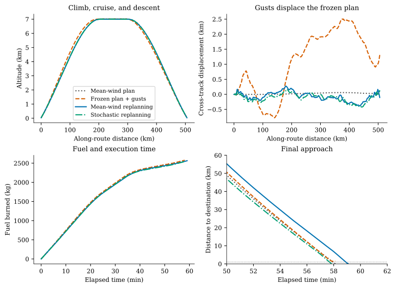
Figure 3:Complete flight profiles for the first paired gust realization. The frozen plan executes the same commands as the mean-wind reference, so both burn the same fuel in this model, but their ground positions differ. Replanning changes commands in response to the observed position and gust. The horizontal line in the final-approach panel marks the 1 km arrival tolerance.
Arrival, fuel, and numerical sensitivity
In the three recorded wind realizations, the frozen plan misses the arrival tolerance each time. Both replanning methods arrive within tolerance in all three trials. Their fuel difference is smaller than the distinction between arriving and missing the destination, so arrival and fuel are reported separately:
| Controller | Fuel (kg) | Arrival error (m) | Feasible arrivals | Largest constraint violation |
|---|---|---|---|---|
| Mean-wind plan | 2577.8 | 66.2 | 1/1 | 0 |
| Frozen plan + gusts | 2577.8 | 2491.3 | 0/3 | 0 |
| Mean-wind replanning | 2587.0 | 102.9 | 3/3 | 1.15e-13 |
| Stochastic replanning | 2560.1 | 110.0 | 3/3 | 1.5e-13 |
The repeated runs use 3 independent gust seeds. The figures show mean and sample standard deviation across those seeds, with individual runs also plotted. The mean-wind plan is one deterministic reference run. Prediction uses 32 candidates, 6 shared wind scenarios, and 2 updates per decision. Arrival tolerances are 1000 m horizontally and 30 m vertically. Constraint residuals and replay differences are available in the downloadable metrics.
| Controller | Mean ESS | Total planning time per flight (s) | Rejected updates |
|---|---|---|---|
| Frozen plan + gusts | 11.7 | 1.3 | 0 |
| Mean-wind replanning | 22.2 | 56.1 | 110 |
| Stochastic replanning | 8.8 | 52.2 | 92 |
Planning times are measured wall-clock times on the build machine; they include validation and vary with competing workloads. Rejected-update counts are totals across the recorded flights. The largest 5 s versus 10 s replay difference is 0.261 m in position and 0.0020 kg in fuel. All vertical arrival errors are below 8.3e-13 m.
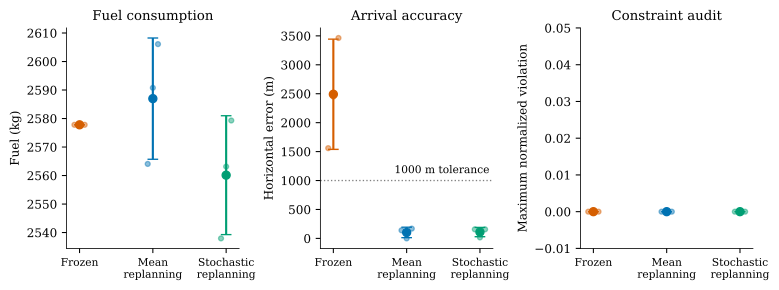
Figure 4:Individual outcomes across three independent gust realizations, with mean and sample-standard-deviation bars. The small trial count supports inspection of these examples; it does not establish a reliable fuel advantage or a failure probability. Tiny residuals near machine precision arise from floating-point integration at the terminal altitude boundary.
Replanning compensates for displacement accumulated under the frozen plan. Whether sampling future gusts also improves fuel consumption depends on the wind model, the trajectory family, and the sampling budget. Conditional-mean replanning is therefore a substantive baseline. A favorable single run is insufficient evidence that the stochastic planner is better.
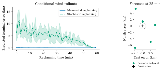
Figure 5:Left: the predicted terminal-error 10th–90th percentile range from the current planning ensemble. The conditional-mean planner has one deterministic future, so its band has zero width. Right: conditional scenario endpoints at one replanning time, with the 1 km arrival region. These small-ensemble ranges are forecast diagnostics, not calibrated confidence regions or constraints.
Increasing the number of candidate samples and increasing the number of wind scenarios address different approximations. Candidate counts of are compared at ; scenario counts of are compared at . Four independent planning seeds are used at the initial full-trip decision. Each resulting plan is evaluated on 128 fresh, shared wind futures that no optimizer saw. This separates variation in the candidate search from variation in the estimated expected cost. Two projected updates need not improve monotonically with either sample count, and this first-decision check does not establish convergence of the entire feedback policy.
The endpoint comparisons in the recorded sweep are:
| Varied budget | Fixed budget | Mean held-out cost at the smaller budget | Mean held-out cost at the larger budget |
|---|---|---|---|
Costs are in kg-equivalent and include large penalties for rare unsuccessful wind futures. They are not fuel totals. In the candidate-count comparison, sample standard deviations across planning seeds are and . Intermediate budgets give nonmonotone results, so these endpoints show sensitivity to sampling budgets without establishing convergence.
The flight diagnostics include fuel, arrival errors, fine-grid residuals, effective sample sizes, accepted and rejected updates, runtimes, and the sampling study. The local replay displays the corresponding paths and observations. To extend the experiment, increase the number of independent realized winds before drawing conclusions about reliability, and compare the gain from a richer control parameterization with the gain from more samples.
Select a controller and replay the recorded flight. The displayed forecast belongs to the most recent planning decision, while the gust display follows the observed realized wind.
Heater Control of a Flow-Through Reactor
The aircraft state contained a few physical quantities and a gust. Many process systems are instead described by fields: the temperature and composition at every point of a vessel. In a flash calciner, clay particles carried by hot gas are heated rapidly while an endothermic reaction converts them into a reactive material that can replace part of the clinker in cement Cantisani et al., 2024. Heaters act on broad regions of such a reactor, while the quantities that matter, such as the conversion of the material leaving it and the highest local temperature, depend on how heat is distributed along the flow.
MPPI needs only the ability to simulate a candidate control sequence and evaluate its cost, and a discretized partial differential equation (PDE) provides both. The number of state values does not enter the update directly: the weights depend on candidate costs, and the update averages control parameters. The state dimension determines the cost of each rollout and how much of the state a few actuators can influence. This section controls a reactor with 4,096 state values through 24 sampled parameters, first planning with the PDE itself and then with a learned surrogate.
A two-field reactor model
Material flows from left to right through a rectangular domain of length 8 m and width 2 m, with measured downstream and across the width. Two fields describe its state: temperature in kelvin and remaining reactant fraction . Conversion is . Both fields are carried by a prescribed downstream velocity , spread by diffusion, and coupled through a temperature-dependent reaction:
The reaction rate has the Arrhenius form s. Converting a unit of reactant cools the material by , and heat is lost toward the wall temperature at rate . Each heater covers one quadrant of the domain, and its input is a fraction of the maximum heating rate . Heater H1 covers the upstream half of the bottom ( m), H2 the downstream half of the bottom, H3 the upstream half of the top, and H4 the downstream half of the top. Material enters with reactant fraction one.
| Quantity | Value |
|---|---|
| Domain and mesh | 8 m 2 m, cells |
| Diffusivity of both fields | m/s |
| Heat-loss rate and wall temperature | 0.01 s, 700 K |
| Reaction cooling | 60 K per unit of reactant |
| Maximum heating rate | 20 K/s |
| Inlet temperature | K |
| Operating limits | K, outlet conversion |
These are teaching assumptions inspired by flash calcination, not calibrated calciner parameters. The model omits separate solid and gas phases, detailed chemistry, residence-time distributions, and industrial geometry.
The Arrhenius factor makes conversion sensitive to temperature. At 950 K the rate is 0.1 s, a time constant of 10 s. At 900 K it falls to about 0.050 s, and at 1000 K it rises to about 0.19 s. Material spends about 40 s in the reactor, so a parcel that remains 50 K colder than its surroundings for part of that time leaves with noticeably more unreacted material. More heating raises the rate, but it also raises the peak temperature, which must stay below 1070 K everywhere. Because the flow speed can vary across the width, the outlet conversion is weighted by flux,
where the sums run over the outlet cells. It must remain at least .
A finite-volume discretization with cells turns the PDE into ordinary differential equations. Advection uses first-order upwind fluxes; diffusion uses centered fluxes with no diffusive flux through the boundaries. An explicit two-stage strong-stability-preserving Runge–Kutta method advances time in substeps of at most 0.1 s. Heater inputs are held for s, and integrating over one control interval defines the transition
which plays the role of the rollout map in Algorithm 1. The mesh partitions physical space; it is not a grid over the 4,096-dimensional state space. Refining it makes each rollout more expensive without changing the number of heater inputs.
Two flow profiles appear below, both with mean speed 0.2 m/s. The field-recovery problem uses a shear flow that is fastest at the center of the channel, m/s with . Material then takes about 36 s to cross the reactor at the center and nearly 50 s near the walls, so a disturbance tilts and stretches as it moves. The surrogate experiment uses uniform flow at 0.2 m/s.
Restoring the operating field
Holding all four heaters at 0.46 for 400 s under the shear flow produces a steady operating state. Its temperature rises from about 800 K at the inlet to a maximum of 1063.54 K, and its outlet conversion is about . Denote its fields by and . Starting from this state, a cold patch enters through the lower part of the inlet:
and otherwise. Control starts at 14 s, when the whole patch has entered the reactor and is traveling through the bottom half where H1 and H2 act. If the heaters stay at 0.46, the colder material reacts too slowly: outlet conversion falls to and remains below the limit for 7.5 s.
The task is to return both fields to the operating state while respecting the limits. The inlet is known to have returned to its normal profile, both fields are measured exactly at each decision, and the PDE is deterministic. As in the derivation of the update, randomness enters only through the candidate controls.
Departure from the operating state is measured by the normalized field error
A cell that is 20 K too cold contributes as much as a cell whose conversion is 0.1 too low. The squared error penalizes warming as well as cooling, so heat delivered to material outside the cold patch counts against a plan. Each heater acts on a quadrant of 512 cells, and four such inputs cannot set the state values independently. Some error must remain until the cold material leaves the reactor.
MPPI plans over intervals, a 40 s horizon equal to the mean residence time. With the control applied during the previous interval, the planning objective is
The second term discourages departures from nominal heating, and the third discourages abrupt changes between intervals. Earlier in the chapter, control effort entered only through the KL penalty and contained state costs. Here plays the role of and includes control terms written in physical heater units. The derivation of used only that assigns a cost to each complete candidate sequence, so these terms change the target distribution without changing the update.
The limits enter in two ways. During sampling, a candidate whose states at the 2 s decision times exceed 1070 K anywhere, or bring outlet conversion below , receives infinite cost and therefore zero weight. In the distributional objective, this restricts the reference to sequences that pass the check. That set need not be convex, so the mean of the resulting Gibbs distribution need not satisfy the limits, as in Exercise Exercise 4. Each proposed update therefore requires its own check before it can replace the stored plan.
Sampling in a bounded control space
A plan contains heater values. Sampling each independently would produce irregular schedules and spend samples on rapid fluctuations that the third term of penalizes. As in the aircraft example, a candidate is described by a few smooth parameters: six knots for each heater, linearly interpolated to the 20 decision times. This gives 24 sampled parameters, collected in a array .
Heater inputs must stay in , while Gaussian samples are unbounded. Clipping would change the distribution of the clipped values, as noted after Algorithm 1. Instead, a logistic map takes latent parameters to physical knot values,
applied elementwise. The array contains the stored plan evaluated at the six knot times, so reproduces the stored plan up to interpolation error. The derivative of the sigmoid is , which is about 0.25 near . A latent change of 0.7, one standard deviation of the sampling distribution below, therefore moves a knot by about , or two percentage points of heating.
Gaussian densities are defined on . The reference is and the proposal is . At each decision the decoder and the reference stay fixed while starts at zero. Each of four updates draws candidates , decodes them, simulates them in the PDE, and computes
This is the importance-corrected update in latent coordinates, with and the mean in place of the nominal controls. The weighting temperature is dimensionless, like , and unrelated to temperature in kelvin. Since latent zero decodes to the stored plan, the KL penalty charges for changing that plan, not for heating as such. This is the alternative, noted with the reference distribution, of centering the reference on a baseline sequence, with the previous plan as the baseline. The average is taken in latent coordinates, so the decoded heater schedule generally differs from the weighted average of the candidates’ physical schedules.
The temperature sets which cost differences matter. At the first decision, the stored plan has . Before correction, a candidate whose cost exceeds another’s by , about of that value, receives half the weight.
The likelihood correction changes the weights substantially once has moved. At the fourth update of the first decision, after three accepted updates, candidate 12 had cost 0.05649 and candidate 180 had cost 0.05840. Exponential cost weighting alone would give candidate 12 about times the weight of candidate 180. Its recorded weight, 0.0682, was instead less than half of candidate 180’s weight, 0.1565. The ratio corresponds to corrected costs that differ by in favor of candidate 180, so the correction term contributes about 0.0102. Candidate 12 lies farther in the direction in which the proposal had already moved, where the proposal samples more often than the reference. Exercise Exercise 6 works through this calculation.
Validating and executing a sampled update
Each update ends by checking the proposed mean. The controller decodes for step fractions in turn, and accepts the first that lowers below the stored plan’s value and passes a finer check. The finer check records the PDE state every 0.25 s over the 40 s plan, followed by another 40 s at nominal heating, and tests both limits at every record. If no step fraction succeeds, both and the stored plan remain unchanged.
After four updates, the controller applies the first 2 s of the stored plan to the PDE, shifts the plan by one interval, and appends nominal heating. The stored plan is the exact heater sequence that passed validation; its six-knot approximation only centers the next round of sampling. Because the plant is the same deterministic PDE with a known inlet, executing the first action reproduces the predicted state. The shifted plan followed by nominal heating then repeats a trajectory that has already passed the finer check, except for its final 2 s. The validation tail at nominal heating is what makes this continuation available: if every later update is rejected, the controller still holds a checked plan. Receding-horizon control develops this property, recursive feasibility, with terminal conditions in place of a simulated tail.
The procedure needs a feasible plan at the first decision. Unchanged heating does not qualify, since it violates the conversion limit. The experiment supplies an initial schedule that holds H1 at 0.50 for 8 s and returns it to 0.46 over the following 8 s, with the other heaters at nominal. This schedule is given to the controller, not found by it; MPPI starts from it and revises it at every decision.
Recorded recovery
All three schedules start from the same disturbed state at 14 s and are recorded until 80 s on a 0.25 s output grid. The integrated field error is , and heating energy is the integral of the mean heater fraction over the same interval. Both are measured in seconds; heating energy counts seconds at full average heating, since the model has no heat capacity to convert it to joules.
| Schedule | Integrated field error | Heating energy | Maximum temperature | Lowest outlet conversion |
|---|---|---|---|---|
| Unchanged heating | 3.709 s | 30.360 s | 1063.54 K | |
| Supplied initial schedule, executed unchanged | 2.098 s | 30.484 s | 1066.94 K | |
| MPPI | 1.962 s | 30.439 s | 1066.16 K |
The supplied schedule alone removes of the integrated error of unchanged heating and restores the conversion limit. MPPI removes , which is less error than the supplied schedule, while using slightly less heat than that schedule and staying 3.8 K below the temperature limit.
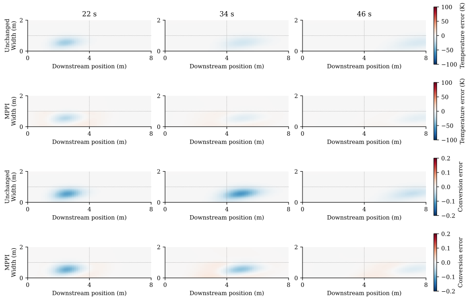
Figure 7:Departures from the operating state at 22, 34, and 46 s. The first two rows show temperature error under unchanged heating and under MPPI; the last two rows show conversion error. Blue marks colder material or lower conversion. Dotted lines mark the heater quadrants. The deficit is carried downstream and tilted by the shear flow. MPPI reduces it, while each heater also warms material around the patch.
The controls in Figure 8 follow the patch. MPPI raises H1 by about five percentage points while the patch crosses the upstream bottom quadrant, then returns it to nominal by about 32 s. Between about 36 and 62 s it lowers H2, by up to 0.8 percentage points near 48 s, as material warmed by H1 passes through the downstream bottom quadrant; the squared error penalizes that excess warmth. The top heaters change by less than one percentage point. Outlet conversion still dips as the patch leaves, but its lowest value is instead of .
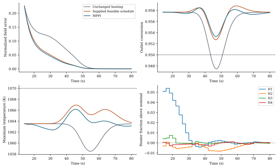
Figure 8:Recovery from the disturbed state at 14 s. Top left: normalized field error . Top right: outlet conversion, with the limit dashed. Bottom left: maximum temperature, with the 1070 K limit dashed. Bottom right: executed MPPI heater inputs relative to nominal heating 0.46, each held for 2 s.
The sampling statistics show how much of this result comes from accepted updates. Over 33 decisions, 24 of 132 updates were accepted. Only four of the accepted updates used the full weighted mean; the other 20 needed a step fraction of or less. Nine acceptances occurred in the first three decisions and eleven more between 32 and 42 s, as the patch approached the outlet. From 44 s on, only 3 of 72 updates were accepted. By then the stored plan was already returning to nominal heating, and random perturbations tended to add error to a field that was recovering on its own. The effective sample size ranged from 19.8 to 64.1 of 256 candidates, and between 108 and 217 candidates per batch passed the constraint check. With the weight concentrated on a few dozen candidates, the weighted mean is a noisy proposal, and the step fractions trade progress for reliability.
The opening decision was also repeated with three optimizer seeds at each of 128, 256, and 512 candidates. All nine runs lowered the objective of the supplied schedule, by between and . The effective sample size grew with the number of candidates, from 4.3–18.9 at 128 to 32.5–63.0 at 512. The final objectives did not improve with the count: their spread across seeds at a fixed count exceeded the differences between the averages at different counts. These repetitions measure optimizer variability at one physical state. They do not establish that the recorded plan is globally optimal.
Planning took 13.9 s per decision on average, including the finer checks and first-use compilation. This is longer than the 2 s control interval: the recording is an offline computation, not a demonstration of real-time control. The numerical model was checked separately by repeating the executed MPPI controls with halved integration steps, which changes the temperature field by 0.0014 K root-mean-square, and on a mesh, which changes it by 0.78 K. The finer mesh reaches 1068.42 K and a lowest outlet conversion of , still within both limits. First-order upwind advection adds numerical diffusion of roughly m/s, much larger than , so part of the visible spreading of the patch is a property of the discretization.
Planning with a learned surrogate
Each recovery decision simulated 256 candidates over 20 intervals in each of four updates, or interval rollouts before validation. For this coarse PDE the budget is affordable. A finer mesh, separate gas and solid phases, or a computational fluid dynamics model of an industrial calciner would make it expensive. A common response is to learn a fast approximate transition model, a surrogate, from simulations and to use it for the candidate rollouts. MPPI requires only rollouts and costs, so the substitution changes no part of the update. It changes which model ranks the candidates: the weights now favor candidates that the surrogate predicts to be good.
The surrogate experiment uses the uniform-flow version of the reactor with a different task. Nominal heating is 0.48 in all four quadrants, and the inlet temperature K fluctuates. The deviation follows the Ornstein–Uhlenbeck model of the aircraft example with correlation time 20 s and stationary standard deviation 15 K, held constant over each 2 s interval and observed at each decision. The objective is economic: use as little heat as possible while keeping outlet conversion at least and temperature at most 1070 K. The planning cost averages, over 20 steps,
where and the conversion and temperature are evaluated at the end of interval .
The surrogate is a residual convolutional network that predicts the change of both fields over one 2 s interval. Its six input channels are the normalized temperature and reactant fields, the map of heater fractions, the normalized inlet temperature, and two coordinate channels. Four convolutions with 16 hidden channels and dilations let each output cell depend on inputs up to eight cells away, more than the 3.2 cells that material travels in one interval. After each predicted step, the reactant fraction is projected onto ; temperature is not modified. Training used 256 PDE episodes of 120 s with varied heating, warm and cold starts, smooth spatial transients, and inlet fluctuations, split by whole episode into 179 training, 38 validation, and 39 test episodes. The loss combined one-step error, five-step rollout error, and outlet error. The checkpoint used here was selected after three epochs of Adam within a local CPU budget.
| Held-out 40 s rollouts, 39 test episodes | Result |
|---|---|
| Temperature root-mean-square error | 4.59 K |
| Outlet-conversion mean absolute error | 0.0039 |
| 95th percentile of peak-temperature underprediction | 8.31 K |
| Largest reactant-fraction bound excess before projection | 0.068 |
These averages must be read against the margins that decide feasibility. Under constant heating, the lowest outlet conversion in the trials below is , a margin of 0.09 percentage points, while the surrogate’s average conversion error is 0.39 percentage points. A plan accepted on the surrogate’s predictions alone could violate the conversion limit in the PDE, and an 8 K underprediction of the peak temperature could hide a violation of the temperature limit.
The controller therefore keeps two roles for the PDE. Every applied control advances the PDE under the realized inlet, and every proposed plan is simulated in the PDE before it is accepted. The planner samples candidates in latent coordinates with and the reference , which now decodes to constant nominal heating. Its KL penalty charges departures from nominal heating, while the proposal mean is initialized from the shifted previous plan. Candidate costs come from surrogate rollouts, and the weights use . A candidate that uses one percentage point less heat on average, with no penalty active, receives about times the weight. After each of two updates per decision, the weighted mean is accepted only if it lowers the surrogate cost and a PDE rollout under the conditional mean inlet keeps conversion at or above and temperature at or below 1070 K at every 2 s output. Otherwise the previous plan is kept. If the shifted previous plan fails the PDE check at the next decision, constant nominal heating is checked instead; if both fail, the episode stops and records a planning failure.
Two forecast variants separate reaction to the observed inlet from planning under its uncertainty, as in the aircraft example. The mean-forecast controller scores each candidate under the conditional mean of the future inlet. The stochastic controller scores it under four conditional futures, shared by all candidates, and averages the four costs before weighting.
Surrogate and PDE planning compared
Eight paired trials start from the warm state and last 160 s. Within a trial, constant heating and both MPPI controllers face the same realized inlet sequence.
| Controller | Mean heating energy | Lowest outlet conversion | Highest temperature | Accepted updates | Planning time per decision |
|---|---|---|---|---|---|
| Constant heating | 76.800 s | 1059.5 K | none | none | |
| Surrogate MPPI, mean forecast | 75.807 s | 1051.9 K | 127 of 1280 | 1.32 s | |
| Surrogate MPPI, stochastic forecast | 75.759 s | 1052.4 K | 143 of 1280 | 4.45 s |
Lowest and highest values are taken over all trials at the 2 s outputs. No episode stopped, and every execution stayed within both limits on the 2 s grid and on a separate 0.1 s audit of the executed controls. Paired differences in heating energy, with Student-t intervals over the eight trials, are s for mean-forecast MPPI minus constant heating, s for stochastic MPPI minus constant heating, and s for stochastic minus mean-forecast MPPI. Both MPPI variants use about less heat than constant heating. The trials do not establish a difference between the two forecast variants. About one proposed update in ten was accepted.
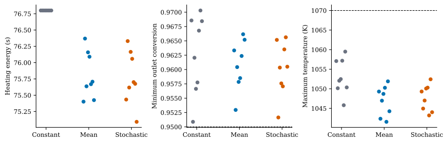
Figure 9:Eight paired 160 s trials of surrogate MPPI in the uniform-flow reactor. Left: heating energy. Center: lowest outlet conversion, with the limit dashed. Right: highest temperature, with the 1070 K limit dashed. Each dot is one trial, and the three controllers in a trial share one realized inlet sequence.
To isolate the effect of the rollout model, the same planner was run from the warm state with zero inlet deviation, once with surrogate rollouts and once with PDE rollouts, using the same random seed and settings. Each resulting 40 s plan was then evaluated in the PDE on 32 fresh inlet futures. The first heater commands were nearly identical, from the surrogate and from the PDE, and the held-out PDE costs were 0.47331 and 0.47250. Planning took 14.57 s with the surrogate and 11.25 s with the PDE, both including PDE validation and the recording of candidate snapshots. For this coarse PDE the surrogate brought no speed advantage. A surrogate pays for itself only when the model it replaces is substantially more expensive to roll out.
The two plans nearly coincide because of the structure of . For a candidate that triggers neither penalty, the cost consists of mean heating and the slew term, which depend only on the controls. The surrogate and the PDE assign such a candidate the same cost. For both selected plans, the cost on the planning forecasts agreed with the held-out PDE cost to within 10-6. Such agreement between different models and inlet futures means that the penalties contributed essentially nothing in either evaluation. The rollout model affects the weights only through the penalties, that is, through deciding which low-heating candidates violate the conversion limit and which high-heating candidates exceed the temperature limit. Surrogate accuracy matters near the boundary of the feasible set, which is also where an economic objective drives the plan. Average errors over held-out trajectories do not measure accuracy there. The PDE acceptance check instead tests the one plan that will be executed, under the conditional mean inlet.
Both experiments use the same structure. Sampling explores a small, bounded parameterization of the heater schedule; exponential weights with a likelihood correction propose an update; and the full model decides whether the update replaces a plan that is already known to be feasible. In the recovery experiment the full model also generates the candidate costs. In the surrogate experiment a learned model generates them, and its errors matter where the constraints are nearly active.
The replay opens on the field-recovery experiment. Play the recording to follow the cold patch under unchanged heating and MPPI, display the error relative to the operating state, or open the sampled control update to see six candidates and their full-batch weights at 14, 22, and 34 s. The Surrogate vs PDE tab compares the learned model with the PDE under identical controls and inlet histories in the uniform-flow experiment. Every field image is a recorded numerical rollout; the page performs no simulation.
Summary and Outlook
MPPI begins with the single-shooting rollout and changes how its candidate inputs are combined. A reference distribution favors small inputs; exponential state-cost weights favor useful trajectories; a Gaussian fit turns the resulting distribution into a stored control sequence. Importance correction preserves the target when samples are drawn around a nonzero nominal sequence.
The aircraft application separates control exploration from wind uncertainty and averages wind costs before assigning a candidate its weight. Increasing the number of candidate controls and increasing the number of wind futures address different estimation errors. Neither guarantees that a weighted mean is feasible or improves the cost, so candidate updates are validated before they replace the stored plan.
The reactor application uses the same update on a discretized PDE with 4,096 state values. Six bounded knots per heater reduce the search to 24 latent parameters, in which the Gaussian densities and the likelihood correction are computed, and candidates that violate a limit receive zero weight. Because the mean of feasible candidates need not be feasible, each proposed update is checked in the PDE, damped when necessary, and otherwise rejected; once the field was recovering, most updates were rejected. Replacing the PDE by a learned surrogate in the sampling loop changes the model that ranks candidates, while the PDE still decides which plan is executed. With an economic objective, the surrogate’s errors matter mainly near the operating limits, which is where the plan operates.
The controller still needs an execution rule. Applying one action, observing the result, and solving again provides feedback even though each stored sequence is open loop. Receding-horizon control develops that rule further, including the choice of horizon, terminal conditions, and feasibility safeguards. These questions apply whether the planner uses derivatives or sampled trajectories.
The method’s name also reflects a connection to expectations over entire stochastic paths. Path-integral stochastic control, after stochastic dynamic programming, develops that connection and states the additional assumptions under which path weighting yields an optimal current feedback action.
Computational Sources
The aircraft and reactor experiments use small numerical modules and read precomputed results when the book is built. The aircraft evaluator averages each candidate’s costs over a shared ensemble of possible wind futures.
Reactor PDE, heaters, and inlet disturbances and shear flow and cold inlet pulse
Convolutional surrogate and surrogate MPPI with PDE acceptance checks
The experiment scripts record the physical parameters, planner settings, seeds, and validation diagnostics alongside their results. The aircraft replay and the reactor replay display recorded simulations without a Python kernel. Regeneration commands are in the repository README.
Exercises
Solution to Exercise 1
(a) The unnormalized weights are , whose sum is . The normalized weights are , giving .
(b) The common factor cancels between numerator and denominator. Direct evaluation would underflow in ordinary floating-point arithmetic. Subtracting the minimum corrected cost before exponentiating recovers the original three weights.
(c) The unique minimum cost belongs to perturbation 1. Its normalized weight approaches one, so . The qualification that corrected costs are fixed matters: a likelihood correction can itself depend on .
Solution to Exercise 2
(a) Up to a constant, the negative log Gibbs density is
Its first-order condition is . All coordinates of its minimizer are equal, giving
The result is independent of the proposal mean because the likelihood ratio cancels the proposal density in the expectation.
(b) Omitting that ratio replaces the reference quadratic by . The corresponding first-order condition is , so its mean is
Thus the two procedures converge to different expectations.
(c) A minimal implementation uses the same perturbations for both estimates so that their difference is easier to observe:
import numpy as np

rng = np.random.default_rng(728)
N, h, r, kappa, lam = 10, 0.1, 1.0, 4.0, 0.5
U = np.full(N, 0.4)
for K in (1_000, 10_000, 100_000):
    eps = rng.normal(size=(K, N)) * np.sqrt(lam / (r * h))
    inputs = U + eps
    cost = 0.5 * kappa * (h * inputs.sum(axis=1) - 1.0) ** 2
    corrected = cost + h * r * (eps @ U)
    estimates = []
    for scores in (corrected, cost):
        weights = np.exp(-(scores - scores.min()) / lam)
        weights /= weights.sum()
        estimates.append((weights @ inputs).mean())
    print(K, *estimates)
The estimates approach 0.8 and 0.88. More samples reduce Monte Carlo error; they do not repair an omitted likelihood ratio. Individual runs need not approach their limits monotonically.
Solution to Exercise 3
(a) For a fixed candidate, averaging the weights estimates , whereas the desired score depends on . The exponential is nonlinear. Favorable gust histories receive disproportionate weight, so this procedure can favor a candidate whose expected cost is larger. The reference-to-proposal correction for control sampling does not remove this difference in the disturbance objective.
(b) The safe candidate has expected cost 1 and exponential score 1. The risky candidate has expected cost 2 but exponential score . Expected cost favors the safe candidate; the exponential score favors the risky candidate.
(c) For each candidate, simulate multiple gust histories and form . Then use as the candidate score in the sampling optimizer. Shared gust histories across candidates can make paired comparisons less variable. As the number of disturbance samples increases, this score estimates the intended expected cost. The subsequent Gaussian mean fit need not minimize that cost over deterministic plans. Finite sampling introduces further error, and an average of feasible plans may violate nonconvex constraints. The proposed plan still needs cost and feasibility checks.
Solution to Exercise 4
(a) The controller executed 0.6. Its shifted initial guess is , and the measured state becomes the initial state for every new rollout. The guess is then updated by sampling; it is not a commitment to execute all three entries.
(b) The mean is , which produces outside both allowed intervals. Feasible samples do not ensure a feasible mean under nonconvex constraints. The implementation should validate the proposal and retain the feasible incumbent when that validation fails, as in the aircraft example.
Solution to Exercise 5
(a) Each of the cells carries a temperature and a reactant fraction, so a rollout advances state values. The weighted mean averages the latent parameters.
(b) One decision simulates intervals. Each interval needs at least substeps, so at least substeps are required, each evaluating the right-hand side twice in the two-stage Runge–Kutta method.
(c) The refined mesh has m, so the advective condition allows s, and the 0.1 s cap remains binding. The state dimension grows by a factor of four, to . The number of sampled parameters stays 24. Each substep updates four times as many cells, so the work per decision grows by about a factor of four. The weights and the update keep the same dimension.
(d) A single 2 s increase of one heater in the middle of the horizon, with all neighboring values at nominal, is not piecewise linear between the six knot times and cannot be represented. MPPI searches only within the knot family, so the recorded schedule is at best a good member of that family. Finite sampling, the Gaussian mean fit, the regularizing reference, and the step fractions limit even that statement, so the result supports an improvement over the supplied schedule, not optimality.
Solution to Exercise 6
(a) Here and . The decoded inputs are and , whose average is about 0.882. The latent mean is , which decodes to 0.9. The controller averages latent parameters and proposes , subject to validation. Both numbers lie in : the sigmoid maps every real number into , and an average of numbers in stays there. They differ because the sigmoid is curved: near the upper bound, equal latent steps produce a smaller increase than decrease.
(b) For Gaussians with a common covariance,
The last term is the same for every candidate and cancels after normalization. Thus . Writing changes the correction only by another common constant, giving the form of the earlier corrected cost, with .
(c) The weight ratio gives the difference in corrected costs,
The cost difference is , so the correction contributes . Hence . The positive sign means that candidate 12 lies farther along the direction in which the proposal mean has already moved. The proposal draws such candidates more often than the reference would, and the correction lowers their weight to compensate.
(d) The Gaussian density belongs to the unclipped sample, so the ratio must be computed for that variable, with clipping treated as part of the deterministic map from samples to controls, as for the aircraft duration. Every sample beyond a bound then produces the same control and the same cost. Those samples are indistinguishable to the weights, and the weighted mean of unclipped values can itself lie outside . The logistic decoder keeps distinct latent samples distinct and always decodes the mean inside the bounds.
Solution to Exercise 7
(a) Without active penalties, reduces to mean heating plus the slew term, both functions of the controls alone. Any rollouts that remain valid therefore give the same cost under either model. Surrogate errors can change the cost only of candidates for which at least one model predicts an active penalty, that is, candidates near the conversion or temperature limit. Minimizing heating pushes the plan toward the conversion limit, so these are the candidates that matter.
(b) No. The 8.31 K figure is a percentile over held-out windows, not a bound: one window in twenty underpredicted by more, and an optimized plan is not drawn from the held-out distribution. Adding 8.31 K to 1064 K already exceeds 1070 K. The PDE acceptance check simulates the proposed plan before it replaces the stored one. It uses the conditional mean of the future inlet, so it does not guarantee feasibility under the inlet that is actually realized. The audit on a 0.1 s grid checks the executed controls only after the fact.
(c) Larger margins make surrogate rollouts reject more candidates near the limits. Fewer proposals then fail the PDE check, and violations under the realized inlet become less likely, but the controller gives up heating reductions that were feasible. Smaller margins allow plans closer to the limits, at the price of more rejected proposals and less protection against surrogate error and inlet uncertainty. Margins calibrated from surrogate errors near the limits, rather than from average errors, would make this choice less arbitrary.
(d) A surrogate reduces planning time when rollouts of the full model dominate the computation and the surrogate is much cheaper to evaluate in large batches, for example with a finer mesh, multiphase physics, or computational fluid dynamics. Removing the PDE check would require evidence about errors near the constraint boundary for the kinds of plans the optimizer proposes, not only average errors on training-like trajectories, together with closed-loop trials whose executed controls are audited in the full model.
Solution to Exercise 8
Answers depend on the training data and budget. Useful comparisons keep the initial state, supplied schedule, planner settings, and optimizer seeds fixed, so that differences come from the rollout model. Since the tracking objective depends on the entire field, surrogate errors affect every candidate’s cost, unlike in the economic objective of Exercise Exercise 7. When the surrogate ranks candidates differently from the PDE, an accepted update can lower the surrogate objective while raising the PDE objective, so both should be recorded for every proposal. For part (c), the fraction of proposals rejected by the PDE check, the gap between the surrogate’s predicted objective and the PDE objective of each proposal, and raw reactant-fraction values outside before projection all signal that the surrogate is operating outside its training distribution.
Self-checks
Solution to Exercise 9
Conditioning a new plan on the observed state supplies feedback. A control sequence computed from many samples and then frozen still executes open loop.
Solution to Exercise 10
Only the candidate controls are random. The PDE is deterministic and the inlet is known after the pulse, so random numbers serve only to explore heater schedules. A different seed changes the sampled candidates and therefore the plan. Across the nine repetitions of the opening decision, the final objective varied by about .
- Williams, G., Drews, P., Goldfain, B., Rehg, J. M., & Theodorou, E. A. (2017). Information Theoretic Model Predictive Control: Theory and Applications to Autonomous Driving. 10.48550/arXiv.1707.02342
- Williams, G., Aldrich, A., & Theodorou, E. A. (2017). Model Predictive Path Integral Control: From Theory to Parallel Computation. Journal of Guidance, Control, and Dynamics, 40(2), 344–357. 10.2514/1.G001921
- Pan, C., Yi, Z., Shi, G., & Qu, G. (2024). Model-Based Diffusion for Trajectory Optimization. Advances in Neural Information Processing Systems, 37. https://proceedings.neurips.cc/paper_files/paper/2024/file/6a5c38a730b17f3827c09cf6b192be04-Paper-Conference.pdf
- Sun, J. (2022). OpenAP.top: Open Flight Trajectory Optimization for Air Transport and Sustainability Research. Aerospace, 9(7), 383. 10.3390/aerospace9070383
- Copernicus Climate Change Service (C3S). (2018). ERA5 hourly data on pressure levels from 1940 to present. Copernicus Climate Change Service (C3S) Climate Data Store (CDS). 10.24381/cds.bd0915c6
- Cantisani, N., Svensen, J. L., Hansen, O. F., & Jørgensen, J. B. (2024). Dynamic modeling and simulation of a flash clay calciner. IFAC-PapersOnLine, 58(14), 283–288. 10.1016/j.ifacol.2024.08.350