The preceding chapters formulated and optimized trajectories through discrete transition maps. Physical models are often given instead by ordinary differential equations, so their states and controls are functions of time. A finite-dimensional optimizer cannot choose an entire function directly. Continuous-time trajectory optimization therefore begins by replacing those functions and their differential equations with finitely many variables and constraints on those variables.
How can that replacement preserve enough of the differential equation to make the resulting trajectory meaningful between the stored time points?
This replacement is called transcription, and the resulting finite optimization problem is a nonlinear program (NLP).
The direct-collocation formulation used here stores state and control values at selected times and interpolates between them with low-degree polynomials. The differential equation is enforced at selected points on each time interval. This chapter develops that construction from one simple example through Euler, trapezoidal, and Hermite--Simpson transcriptions, then applies it to the motion of an overhead crane.
A One-Interval Example
How can a constraint on four endpoint values ensure that the chosen control produces the required displacement?
Consider a point that must move from to . Its velocity is the control, so
and the objective penalizes squared control effort,
Both and are unknown functions. As a first finite approximation, retain only their endpoint values and let the control vary linearly between and . Integrating means that the change in state equals the area under this control. The shaded region below is a unit-width trapezoid. Its area is the average of its two endpoint heights, and , multiplied by the width.
Figure 1:Drag the endpoint controls or play the accumulation from left to right. The shaded rectangle and triangle sum to the state change implied by . Setting the interval width to gives the state-change relation .
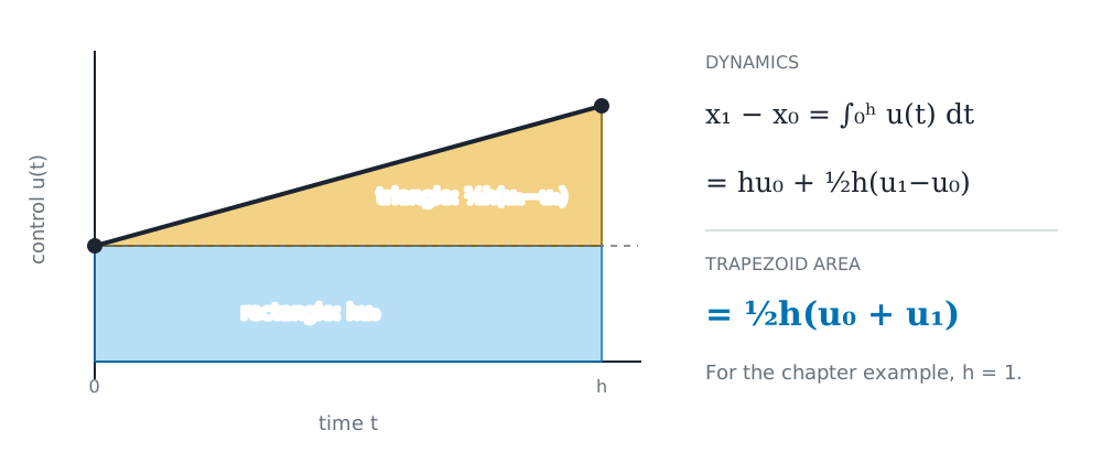
Figure 2:A linear control connects and across an interval of width . The rectangle and triangle sum to . Because , this area equals .
The optimizer must choose endpoint states and controls that agree with this area calculation. Otherwise, it could choose and while setting both controls to zero: the endpoint conditions would hold, but zero velocity could not produce the displacement. To exclude such choices, the stored state change must equal the change predicted by integrating the control. Moving both quantities to the left gives the constraint
The left-hand side measures the mismatch between these two changes and is called the defect. Requiring that mismatch to vanish gives a defect constraint, which enforces the dynamics within the chosen approximation. The equation is algebraic because it relates the four numbers through arithmetic operations; there is no unknown function to differentiate or integrate when evaluating it. An optimizer can therefore check the constraint directly for each candidate set of endpoint values.
Approximating the running-cost integral by the average of its endpoint values gives the finite nonlinear program
The defect integrates the linear control exactly. The objective uses another approximation: is generally quadratic, so averaging its endpoint values need not give its exact integral. Both calculations become exact for a constant control.
The boundary conditions reduce the defect to . Substituting into the objective gives
The squared term is minimized at , which also gives . The resulting interpolation is the exact solution and .
This example already contains the main ingredients of direct collocation. The function values became optimization variables, integration became a weighted sum, and the differential equation became an equality constraint. The remaining sections construct these operations systematically for nonlinear vector dynamics and higher-degree polynomials.
From a Continuous Problem to a Finite NLP
Which quantities and constraints must a transcription retain from the continuous-time control problem?
We retain the earlier notation for the state, for the control, and for cost. Here is continuous physical time, while will index mesh intervals. The running cost is a cost per unit time; integrating it over an interval produces the counterpart of the discrete stage cost . The terminal cost is written because the final physical time is . Scalar examples omit boldface.
With inequalities and equalities , the continuous-time Bolza problem is
The equality imposes endpoint conditions, while imposes constraints along the path, such as actuator limits or a bound on the state. A fixed final time is supplied as data and omitted from the decision variables. Setting gives the Mayer special case, while setting gives the Lagrange special case. All three forms use the same transcription.
Two transcription strategies differ in which values become decision variables and in how they impose the differential equation:
| Strategy | Finite decision variables | Treatment of the ODE |
|---|---|---|
| Shooting | Control parameters and, in multiple shooting, selected boundary states | A time integrator advances the state sequentially inside each shooting interval |
| Direct collocation | State and control values at selected nodes | Algebraic defect equations enforce the ODE simultaneously |
Shooting and collocation are therefore distinct transcription strategies. A collocation method may reproduce a familiar integration formula, but it exposes the state values to the NLP rather than hiding every state update inside a simulation. The term direct indicates that the continuous problem is converted directly into an optimization problem, without first deriving necessary conditions such as the Pontryagin equations.
To apply a local approximation repeatedly over the horizon, divide time into intervals with endpoints
This sequence is a mesh, with indexing its intervals. We write and for values at mesh time , as in the earlier discrete-time chapters; the subscript is an index, not a physical time. On each interval, the normalized coordinate is , or equivalently
Every physical interval is thereby mapped to the same reference interval . Differentiation and integration formulas can be constructed once on this reference interval; the length then supplies the physical-time scaling. If the final time is also optimized, the interval lengths become variables or fixed fractions of the variable horizon; the reference-interval operators remain unchanged.
Polynomial pieces on a time mesh
A single polynomial can represent a trajectory over the entire horizon; the opening example’s solution already does so. Why introduce several pieces? Consider the same scalar dynamics , starting from , but now moving right at unit speed until and then left at unit speed:
The state is continuous, but its slope changes abruptly at the switching time. Two line segments represent it exactly. A single polynomial has a continuous derivative, so it cannot reproduce this corner exactly, although it can approximate the trajectory. The ODE here holds on either side of the switch; the control’s value at that one instant does not affect its integral.
The comparison below uses the quadratic , which passes through the same states at . Matching these three values does not reproduce the motion between them: the quadratic has a continuously varying slope, while the prescribed velocity switches from +1 to -1.
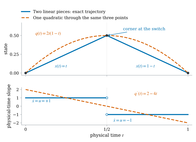
Figure 3:Two linear pieces represent the prescribed motion exactly. The dashed orange quadratic matches the three black sample points but differs between them. The lower panel compares their physical-time derivatives. Open circles indicate the two one-sided slopes at the switch, where the exact state has no derivative. Higher-degree global polynomials can improve the approximation, but every single polynomial has a continuous derivative.
Even when the trajectory is smooth, some portions may change much faster than others. Separate polynomial pieces let us shorten the mesh intervals near a rapid change while retaining longer intervals elsewhere. Increasing the degree of one global polynomial adds flexibility across the whole horizon. The local representation also gives the optimizer useful structure: each interval’s dynamics constraints involve only values on that interval and neighboring endpoint states. A global polynomial couples values across the horizon through its differentiation matrix.
For a trajectory that is smooth throughout the horizon, a single polynomial of sufficiently high degree can be an efficient choice. Piecewise polynomials give us local control over resolution, allow changes in slope at joins, and keep the constraint derivatives sparse. They require us to connect adjacent pieces explicitly so that the state remains continuous.
We therefore represent the trajectory by a separate polynomial on each mesh interval . The full approximation is piecewise polynomial. To construct the piece on interval , use its local coordinate , where , and write
Thus is the state at the start of this interval and is the state at its end. On the next interval, the local coordinate starts again at zero, and a different polynomial describes the trajectory. The reference interval and its integration weights can be reused even when the physical intervals have different lengths.
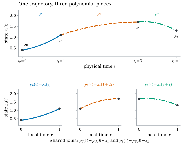
Figure 4:A scalar example of the piecewise representation. The upper panel joins three quadratic pieces on physical intervals of lengths 1, 2, and 1. The lower panels show those same pieces in their own coordinates , preserving their colors and line styles. The middle piece uses , so two units of physical time occupy one unit of local time. Black dots mark endpoint states; matching the right value of one piece to the left value of the next keeps the trajectory continuous. The slopes need not match across joins.
One Polynomial, Two Coordinate Systems
Should a polynomial trajectory be stored by its coefficients or by its values at selected points, and how are the two descriptions related?
The opening example stored a linear control by its two endpoint values. Each piece of a collocation trajectory needs a similar reconstruction: given the values the optimizer stores, what curve do they define between nodes? Start with a scalar polynomial on the reference interval . The construction applies to each state and control component.
Suppose and , and restrict to degree at most one. A line has the form . The first endpoint condition gives , and the second gives , so . Substitution and regrouping give
The weights and enforce the two endpoint conditions: at 0, the formula returns , and at 1, it returns . Between the endpoints, the weights vary continuously; at , for example, the value is . This is the unique line through the two prescribed values. Without the degree restriction, other curves could pass through them. Even for this same line, is an equivalent representation. The weighted form is convenient because each stored value has its own function that determines its contribution throughout the interval. The functions and form a basis for linear polynomials, just as 1 and do. In the first basis, the coefficients are the endpoint values ; in the monomial basis, they are and .
Higher-degree pieces use the same idea with more stored values. To specify which curves those values may define, restrict the degree to at most . The resulting polynomial space is
This space, denoted by , has dimension . Choosing a basis gives coefficient coordinates
The monomial choice gives the familiar expression . A different basis changes the coefficients used to describe the same function.
The same polynomial can instead be identified by its values. Choose distinct points
and record
These points are called support nodes, or interpolation nodes: once the degree is restricted to at most , the stored values determine the whole polynomial. Storing values is useful for trajectory optimization because a bound on the state at a node then becomes a bound on a decision variable. To evaluate the dynamics between nodes, however, we need a formula that reconstructs the polynomial from those values.
With more nodes, the same construction needs one weight function per stored value . To recover at its own node without altering the values at the other nodes, must equal one at and zero at every other support node. A polynomial with those zeros contains the factors for all . Dividing their product by its value at makes the value there equal to one. This constructs the Lagrange basis function, also called a cardinal function,
At a support node , one factor in the numerator is zero unless . When , every numerator equals its corresponding denominator. Consequently,
where the Kronecker delta is shorthand for one when and zero otherwise. This identity specifies the values at the nodes only. At any other , the product formula gives a smoothly varying polynomial weight, which can be negative or exceed one for higher degrees. Thus, unlike a line between two endpoint values, a higher-degree interpolant can take values outside the range of its stored values. The cardinal functions reconstruct the polynomial throughout the interval by
At a node , all terms except vanish. Between nodes, the weighted sum supplies the intervening values. This expression is the Lagrange form of . When the values are prescribed and is constructed to pass through them, is called the Lagrange interpolating polynomial. Each is one basis function; is their weighted sum. Changing one stored value by changes the curve by , so the same function describes how that variable affects the entire polynomial.
The uniqueness of this reconstruction follows from a basic root-counting argument. If two polynomials in have the same nodal values, their difference has distinct roots. A nonzero polynomial of degree at most cannot have that many roots, so the two polynomials must be identical.
Consequently, every polynomial in has a unique expansion in . These functions form the Lagrange basis associated with the chosen support nodes. Its coefficients are exactly the nodal values . Storing a polynomial by its values is therefore also a basis representation, with the basis chosen so that its coefficients have a direct interpretation as function values.
For a scalar polynomial, collect the coefficients and values into column vectors and . The coefficient and nodal descriptions are related by the evaluation matrix
Distinct support nodes make invertible by the same root-counting argument. Thus and are two coordinate vectors for one polynomial, rather than two different approximations.
For example, take and the nodes . In monomial coordinates,
whereas the nodal coordinates are
In the Lagrange basis for these three nodes, the same quadratic is
Here select the nodes , respectively. Both coefficient vectors describe the same quadratic. The transcription used here chooses coordinates like for the state and control: values that can be inserted directly into the dynamics, cost, and bounds. Monomial coefficients remain useful for deriving formulas that act on those values.
Polynomial spaces, bases, and nodes
The construction separates three decisions that are easy to conflate:
The polynomial space specifies which functions are available.
The basis specifies coordinates for a member of that space. Monomial and Lagrange bases span the same .
The nodes specify where values, residuals, or integrals are evaluated.
Changing the basis does not change the exact polynomial space, although it can change numerical conditioning. Changing the nodes changes the interpolation and the operators built from it. The node families introduced later can still use Lagrange nodal coordinates in the NLP.
Polynomial Interpolation and Least-Squares Regression
When should a polynomial pass through every supplied value, and when should it approximate those values with a smaller number of coefficients?
Interpolation and polynomial regression impose different requirements on the same data. Six values at six distinct nodes determine one polynomial of degree at most five that passes through every point. If the values are noisy observations and the aim is to estimate a quadratic trend, a quadratic will generally be unable to pass through all six. Least-squares regression then chooses its three coefficients to minimize the sum of squared discrepancies. The figure below applies both choices to the same six points. Write for the basis evaluation matrix, as in . It has six rows in both cases, but six columns for the degree-five interpolant and three for the quadratic fit.
| Polynomial interpolation | Least-squares regression | |
|---|---|---|
| Input | Exact value conditions | Usually noisy or overdetermined observations |
| Algebraic problem | Satisfy exactly | Minimize |
| Residual | Zero when the value conditions uniquely determine a polynomial | Generally nonzero |
| Typical purpose | Represent a function from exact nodal data | Estimate a trend or conditional mean |
If is square and invertible, minimizing the squared residual also returns the exact interpolant. The two procedures coincide in that case because the chosen polynomial space can satisfy every value condition.
Figure 5:Two polynomials fitted to the same six points (black dots). The solid blue degree-five interpolant passes through every point. The dashed orange quadratic regression minimizes the sum of squared residuals, shown as gray vertical segments. The polynomial degrees differ because a quadratic generally cannot satisfy all six value conditions exactly.
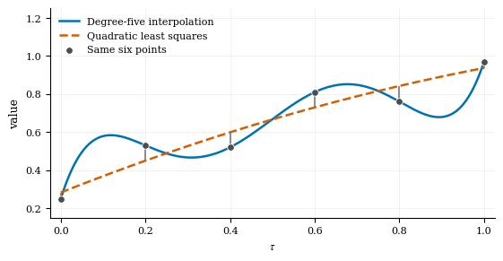
In a nodal state representation of direct collocation, the stored states are unknown decision variables rather than observations. Each candidate vector of support values defines one interpolating polynomial exactly. The optimizer selects a candidate whose ODE residual vanishes at the collocation nodes. A numerical solver may temporarily work with a scalar measure of constraint violation, but the collocation conditions remain equality constraints rather than a statistical regression loss.
Fixed Operators from Nodal Values
How can the stored values give us both the slopes and the integral of every candidate polynomial?
The nodal representation also turns differentiation and integration into matrix and vector products. Once the nodes are chosen, the required arrays can be computed once and reused for every candidate trajectory. The optimizer can then evaluate slopes and integrals as it changes the nodal values, without recomputing those arrays. Each cardinal function is a known polynomial, so its derivative and antiderivative can be computed in closed form by changing its coefficients. Constructing the arrays therefore does not require finite-difference approximations or numerical quadrature of the basis functions. The resulting operators are exact for the represented polynomial, apart from floating-point error in their construction and application.
This is possible because the cardinal functions stay fixed while only their coefficients change. In the representation
each is constant with respect to , so differentiation acts only on . To obtain the slopes needed by the ODE, differentiate and then evaluate at a node :
while integration over the reference interval gives
The resulting differentiation matrix and integration weights depend only on the chosen nodes. Their entries record the derivatives and areas of the fixed cardinal functions. Multiplication by the current nodal values combines these contributions into the derivative or integral of the current polynomial. This is how the transcription supplies the calculus needed by the dynamics and cost through arithmetic on the decision variables.
For a concrete construction, suppose a quadratic is stored by its values at , where denotes the midpoint. The desired outputs are its slope at each of these nodes and its integral over . To build the arrays that return those outputs for any choice of the three values, first construct the three cardinal functions multiplying them:
These are the three contributions in . Their derivatives are , , and . At the left endpoint they give the weights , so . Evaluation at the midpoint and right endpoint supplies the other two rows of the differentiation matrix:
Thus a matrix-vector product turns the three stored values into the three nodal derivatives. Integrating the same cardinal functions gives
The row turns the same three values into the exact integral of their quadratic interpolant. The matrix differentiates every polynomial in exactly, and integrates every polynomial in that space exactly. “Fixed operator” means that these arrays remain constant while the NLP changes the nodal values.
For the earlier polynomial , the stored values are . Applying the arrays gives
The first result agrees with at the three nodes; the second agrees with the integral of over . The figure collects the coordinate change and these two operations for that same polynomial.
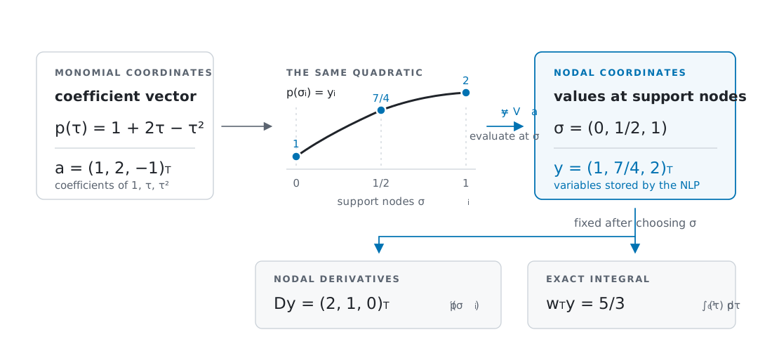
Figure 6:One quadratic, two coordinate systems. Evaluating the monomial coefficients at the support nodes gives . Direct collocation stores the nodal vector ; the fixed operators and then return its nodal derivatives and exact integral without adding optimization variables.
A transcription may use nodes for three distinct purposes:
| Node role | What it does |
|---|---|
| Support node | Supplies a value used to define a particular polynomial by interpolation |
| Collocation node | Specifies where the reconstructed state must satisfy the ODE |
| Quadrature node | Supplies a point used to approximate an integral |
A method often reuses one set of points for two or three roles. Support nodes belong to a particular polynomial: the state, control, and slope polynomials need not use the same interpolation nodes. For example, a state polynomial can be supported at one set of nodes and differentiated at different collocation nodes. In the integration construction below, the collocation nodes also serve as support nodes for the slope polynomial. Both integration and differentiation forms have collocation nodes. Their algebraic residuals differ: one matches state values after integrating slopes, while the other matches slopes after interpolating state values.
From Nodal Slopes to Collocation Constraints
How do those fixed maps convert differential equations into algebraic constraints at the chosen collocation nodes?
The preceding operators apply to any polynomial. A trajectory must also satisfy the dynamics. On each interval, the construction will interpolate the slopes supplied by the ODE and integrate them from the stored left state. Constraints will then require the stored states to agree with the resulting polynomial.
Interval extends from physical time to and contains one polynomial piece. Its local time coordinate runs from at the left endpoint to at the right endpoint. Choose distinct collocation nodes on . A node specifies one time within this interval, ; for example, specifies its midpoint. The state and control values at that time are and .
This evaluation point, together with its state and control values, is called a stage. A stage is associated with a single time, so it has no separate beginning or end. The index identifies the interval and identifies a stage in that interval. Depending on the method, stages may be interior points or may coincide with an endpoint: places a stage at the start and places one at the end. At each stage, the differential equation prescribes the physical-time slope
for . The figure below shows one such evaluation for the scalar dynamics . The state and control are read at the same physical time; the ODE then gives the slope that the state polynomial must match there.
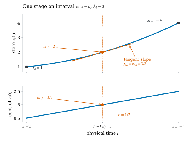
Figure 7:A stage combines a time, a state value, and a control value. Here , , and , so the stage occurs at physical time 3. The orange dots mark and . For , the prescribed slope is , drawn as a dashed tangent in the upper panel. The curves are and . Both panels use physical time; in local coordinates the derivative is .
As before, denotes the state piece in normalized time. Here is the Lagrange cardinal function for the slope nodes ; the slope values determine a polynomial of degree at most . Interpolating them gives the physical-time derivative on this one interval:
This polynomial agrees with each sampled slope at its collocation node. Each sample was evaluated at a stored stage state ; the state curve recovered by integration need not yet pass through those stored states. The stage equations below will enforce that agreement. To recover state values from these slopes, we need to reverse differentiation. For example, both and have derivative . Each is an antiderivative of : differentiating it returns that function. Adding any constant gives another antiderivative, because the derivative of a constant is zero. The slopes therefore determine changes in state, but a starting value is needed to determine the state itself. This starting value fixes the integration constant.
The fundamental theorem of calculus connects antiderivatives to definite integrals. For a scalar function with a continuous derivative, it states that integrating the derivative between two points gives the difference between the function values:
Here is a dummy variable that runs over the integration interval; specifies where that interval ends. Over a short interval of width , the change in is approximately . The definite integral is the limit of sums of these signed changes as the interval widths approach zero. Adding to this accumulated change recovers the value at . Polynomial derivatives are continuous, so the theorem applies to the pieces used here. For a vector state, the same identity applies to each component.
The sampled slopes are derivatives with respect to physical time, whereas is expressed in local time. Since , the chain rule gives
The factor accounts for the duration of the physical interval: a change of in local time corresponds to units of physical time. For example, a constant physical slope acting from 0 to changes the state by .
Applying the fundamental theorem with the left-endpoint condition now gives the state piece:
The final expression follows by substituting the slope polynomial and integrating its terms separately; the stage slopes are constant with respect to . At , every integral vanishes, leaving . Differentiating the expression returns the prescribed slope polynomial. Thus the stored left state selects the unique antiderivative with that starting value. Integrating a polynomial of degree at most gives a state piece of degree at most .
For the scalar example above, and the physical-time slope is , so . Starting from gives
The brackets mean evaluating the antiderivative at the upper limit and subtracting its value at the lower limit. At , the accumulated change is 1, so . At , the accumulated change is 3, so . These are two evaluations of the same polynomial: both integrals begin at the left endpoint, but one stops at a stage and the other at the right endpoint.
This integration is exact for the interpolated slope polynomial. It does not generally give the exact solution of the original ODE: between collocation nodes, the interpolated slope can differ from .
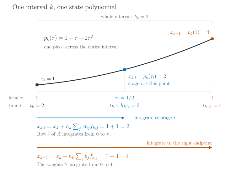
Figure 8:Two integration limits on one polynomial piece. Here , , and . The circle marks stage at , corresponding to physical time 3; the squares mark the interval endpoints. The blue span accumulates a state change of 1 from to , giving . The orange span accumulates a state change of 3 from to 1, giving . The arrows mark integration spans, not successive steps of a numerical solver. The changes come from integrating the derivative of the state curve shown. Only stage is highlighted; each sum uses all the slope stages on the interval.
The integration construction already determines the derivative at each collocation node. Because , any candidate stage values give
This identity holds by construction, before the NLP constraints have been satisfied. It does not yet guarantee that the reconstructed curve satisfies the ODE: the dynamics on the right are evaluated at the stored state , which may differ from the curve’s value .
The remaining condition is agreement between these two state values. The point must lie on the graph of . Imposing at every stage of every interval gives the stage equations
Their coefficients are
Each stage equation therefore sets a state-matching residual to zero:
Once this residual vanishes, the stored state used to evaluate is the state on the reconstructed curve. Substituting into the derivative identity above then gives the ODE at that node. Thus the integration form enforces the ODE at collocation nodes even though its explicit stage residuals compare state values rather than slopes.
For example, consider on an interval of length , starting from , with one collocation node at . A trial stage value supplies the slope and hence the state piece . Its midpoint value is , not the stored value 3. The polynomial’s slope is 3, but the ODE evaluated on the curve at the midpoint asks for . The state equation instead gives . The reconstructed polynomial is then , whose midpoint state and slope both equal 2. The state-matching constraint has made the ODE hold at the collocation node.
Row of integrates each slope basis function from 0 to . Here selects the destination stage and runs over all slope stages that contribute to the polynomial. All these integrals start at 0, including when ; they do not start at the preceding stage. The stage equations are simultaneous constraints, since the slopes on the right depend on the state and control variables being chosen.
For example, take three slope stages at and fix the destination . Every integral in row 2 of now ends at . Varying selects the basis function being integrated: , , or . Figure 9 shows these three signed areas. Although the third slope is evaluated at the right endpoint , its basis function is nonzero between 0 and . That slope therefore contributes to the midpoint state as well. The sum runs over all , not only stages with .
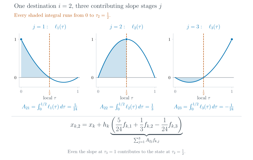
Figure 9:Fixing chooses the integration endpoint; varying includes every slope basis function. For nodes , the blue curves are , , and . Each blue point marks the node where its basis function equals one. The orange dashed line marks the common upper limit . The shaded signed areas form row 2 of : . The third area is negative because lies below zero on this span; it is not absent just because stage 3 lies after the destination. The bottom equation expands the sum for a scalar state; the same coefficients multiply vector-valued slopes in the general case.
The right endpoint has local coordinate 1. Evaluating the same polynomial there uses the full integration span , in place of the span used for stage . Requiring this value to equal the stored endpoint state gives
The coefficients integrate the cardinal functions over the full reference interval. In code, both and are obtained by forming an antiderivative polynomial and evaluating it at the integration limits. No repeated integration of the nonlinear dynamics is involved in computing these coefficients. The worked calculation in A reusable coefficient generator and residual evaluator shows the coefficient arithmetic. If a stage lies at , then for every , so its stage equation gives the same polynomial value as the endpoint equation. Its state must therefore equal ; an implementation can share that variable.
The endpoint equation is a defect constraint: it requires the stored endpoint to match the endpoint obtained by integrating the slopes of piece . The next piece starts from that same stored value, so the two pieces meet:
This shared variable enforces state continuity across the join. If an implementation stores separate endpoint variables for the two pieces, it must impose an equality between them. Choosing an endpoint as a collocation node does not by itself join the pieces. Continuity of the state also does not require continuity of its derivative; neighboring pieces can meet with different slopes.
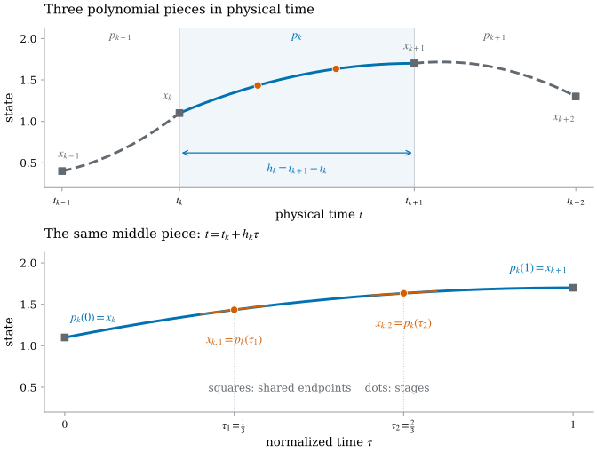
Figure 10:A scalar trajectory consists of polynomial pieces joined at shared endpoint states (squares). The middle piece is shown in blue in both panels; only its time coordinate changes. The stage values (orange dots) lie at and . Tangent marks in the lower panel have slopes because that axis uses normalized time. The stage equations place the dots on the piece, and the endpoint defect makes it reach , where the next piece begins. This schematic uses quadratic state pieces and linear slope interpolants.
The running-cost integral can be treated by exactly the same construction. As in the earlier Bolza-to-Mayer reduction, introduce a scalar state that records the cost accumulated since :
The original objective is now . The augmented state has two rates of change: supplies the physical state rate and supplies the cost rate. Applying the same collocation method to this augmented ODE evaluates both rates at each stage’s state, control, and time. In particular, the cost rate at stage of interval is
Let and denote the accumulated-cost values at the interval’s left endpoint and at stage . Integrating the cost-rate interpolant to a stage and to the right endpoint gives
These are the same stage and endpoint equations as for , with in place of . The increase in accumulated cost across interval therefore supplies its contribution to the discrete objective:
Here is the piecewise control approximation. The single-index is an interval cost, whereas is a sampled cost rate; the factor gives them different units. The weighted sum integrates the polynomial interpolating the sampled cost rates exactly. It approximates the running-cost integral because the composed function need not itself be that polynomial. Such a weighted-sum approximation is called a quadrature rule.
Since , summing the interval increments gives . The accumulated-cost variables can therefore be eliminated and the sum used directly in the objective. Introducing explains why applying one collocation scheme to both rates uses the same nodes and weights; it does not require adding cost variables to the implementation. A different quadrature rule is also possible, with the state and control polynomials evaluated at that rule’s nodes.
Choosing a polynomial for the control
The state and control play different roles. The ODE constrains the state’s derivative, so integrating an interpolant of slopes gives a state polynomial of degree at most . There is no corresponding ODE for the control in this problem. Its representation is a separate choice: a constant command on each interval, a line between endpoint commands, or a higher-degree polynomial.
For example, with two endpoint slopes the state polynomial is quadratic. The control can still be the line
These degrees need not match. Also, substituting polynomial state and control curves into a nonlinear need not produce a polynomial. Collocation matches the state derivative to at the chosen nodes, rather than requiring the ODE to hold identically between them.
To make the control choice explicit, select distinct control support nodes and construct their cardinal functions . The decision variables are control values at these support nodes:
Thus the stage controls are computed from the control variables; they are independent variables only when the representation allows independent values at all those stages. For a constant control, and every entry of is one. For a linear control supported at , row of is .
Using more control support values than collocation stages leaves some control variations invisible to those stage samples. The examples below use ; a richer control representation needs additional sampling or other constraints to account for those variations.
The ODE requires continuous states, but it can admit controls that jump between intervals. Independent control polynomials therefore need no continuity constraint unless the model or chosen parameterization requires one. Sharing endpoint controls between neighboring linear pieces enforces continuity. With separate local variables, the equivalent equality is
At a jump, endpoint stages use the control belonging to their own interval. Finally, bounds on support values guarantee bounds throughout a constant or linear control segment, because its values are convex combinations of its endpoints. A higher-degree polynomial can overshoot those values, so support bounds alone no longer give that guarantee.
Assembling the nonlinear program
The state and control representations now specify which quantities the optimizer chooses and which it evaluates from those choices. The mesh states are shared decision variables at the ends of interval . The stage states are decision variables at the collocation nodes; a stage at an endpoint can use the mesh state itself. For the control, the optimizer chooses the support values at . Evaluating the control polynomial at gives . Together with and the time , this evaluated control supplies the inputs to and .
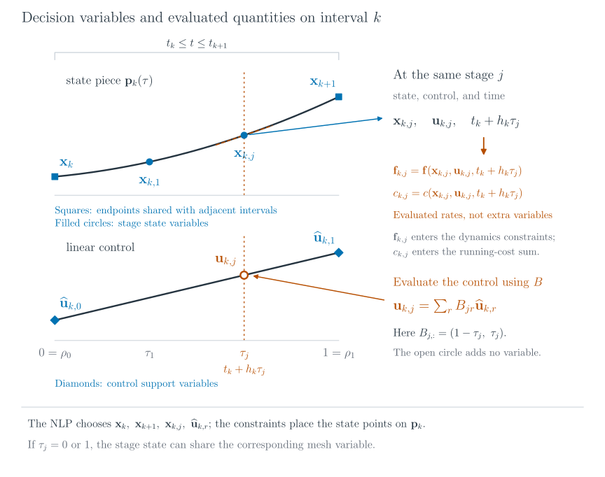
Figure 11:Decision variables and evaluated quantities on one interval. The curves show a scalar example with two collocation nodes, and ; the highlighted stage is . Squares mark mesh states shared with neighboring intervals, and filled circles mark stage states. Diamonds mark the independent control values at and . For this linear control, evaluates the open circle from the two diamonds. The quantities and are then evaluated at the stage state, control, and physical time. Filled blue markers are decision variables; the orange control value and rates are computed from them. The curves depict a feasible choice: the stage and endpoint constraints place the state variables on the integrated polynomial. If a collocation node is an endpoint, its stage state can be identified with the shared mesh variable.
Collect the independent state and control values across all intervals into the decision vector
Here stacks the listed vectors into one column, omitting duplicate variables when a stage shares a mesh endpoint. Stage controls are evaluated using , and any chosen control-continuity equalities are added to the constraints. If is optimized, it is included in as well. The resulting finite optimization problem has the form
In the preceding chapter’s NLP notation, is this scalar objective, stacks the stage, endpoint, and boundary equalities, and stacks the sampled path and bound inequalities. The slope is a vector, distinct from .
The original path and bound constraints apply at every continuous time. This NLP imposes them at selected points, usually its support or collocation nodes. Feasibility at those nodes does not rule out a violation between them. Checking the polynomial between nodes and simulating the chosen control provide complementary diagnostics, developed below.
Every interval constraint touches only local stage variables and neighboring endpoint states. Consequently, most derivatives of the constraints with respect to the decision variables are zero. With variables ordered by time, the nonzero blocks lie near the diagonal of the Jacobian, the matrix of constraint derivatives. NLP solvers can exploit this sparse, block-banded pattern. The arrays and are numerical constants computed before optimization.
Equivalent differentiation form
The differentiation form uses the same collocation nodes as the integration form. It changes which consistency condition is built into the representation and which must be enforced by a residual. The integration form constructs a curve whose nodal derivatives match the evaluated stage slopes, then constrains its values to match the stored stage states. The differentiation form constructs a curve from state-support values, evaluates its stage states directly on that curve, and constrains its derivatives to match the ODE.
To represent the same state polynomials, retain the same degree. The integral of the degree- slope polynomial has degree at most , so take and choose support nodes for the state polynomial. Write for their cardinal functions to distinguish this support-node basis from the slope-node basis . Denote the support values by ; these need not be the stage values at :
At a collocation node , the state is a weighted sum of its support values, and its derivative with respect to is another weighted sum. The fixed arrays containing these weights are
The th row of computes , the point on the state polynomial that we supply to the dynamics function. The th row of computes , the tangent slope measured per unit of local time . Both calculations use the same stored support states ; they do not introduce new decision variables. In particular, the stage state is defined as . State-value consistency therefore holds for every candidate support array; there is no separate state-matching residual at a stage.
To compare this tangent slope with the rate returned by , both must be measured in physical time. A local-time increment corresponds to a physical-time increment . We therefore divide the local-time slope by to obtain the physical-time slope: this is the chain rule used earlier. The remaining constraint sets the physical-time slope residual to zero:
Both slopes are evaluated at the same point on the state curve. Unlike state-value consistency, their equality is not built into the state interpolant. Writing these evaluations using and multiplying by gives
The left side is the polynomial’s slope with respect to ; the right side is the ODE’s physical-time rate multiplied by . The scalar quadratic in Figure 12 shows both calculations at a collocation node that is not a support node.
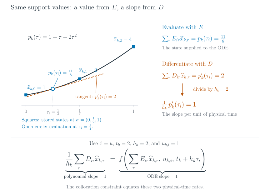
Figure 12:Evaluation and differentiation of the same state polynomial. The support states at define . At the highlighted collocation node , computes the state , while computes the tangent slope . With , the physical-time slope is . For the dynamics and stage control , the ODE also returns 1, so the collocation constraint holds at this node. Taking places the node at physical time .
In matrix shorthand, all nodal constraints are . Here has support states as rows, and has stage slopes as rows; neither is a single state vector. Evaluation at the two ends connects this polynomial to the shared mesh states:
When support and collocation nodes coincide, the cardinal property makes select the corresponding stored state directly. The slope-value and state-value forms describe the same polynomial construction; one integrates nodal slopes, while the other differentiates nodal states.
This implementation pattern is standard in direct collocation Kelly, 2017Andersson et al., 2019. The official CasADi direct-collocation example constructs fixed differentiation, endpoint, and quadrature arrays from Lagrange polynomials, while the NLP variables remain state and control values.
In the integration form, matching the evaluated stage slopes is built into the polynomial construction, while matching the stage states requires constraints. In the differentiation form, matching stage states to the curve is built into evaluation, while matching ODE slopes requires constraints. Both forms also connect the polynomial to the shared mesh endpoints. With the same collocation nodes, state degree, and control representation, their zero residuals describe the same collocation trajectories, although their residual values need not agree for an infeasible candidate. The node-to-NLP recipe for the differentiation form is developed in Constructing the differentiation form from its nodes.
Low-Order Transcriptions
Which familiar integration rules appear when the polynomial and node sets are reduced to their lowest-order choices?
The general construction becomes concrete when only one or two slope values are retained on each interval. These cases recover familiar integration formulas, but the formulas now appear as constraints inside an NLP. For the concrete problems below, fix the mesh and final time. The boundary map includes the prescribed initial state and any terminal conditions; includes path constraints and state/control bounds. Each displayed program specifies the points where those inequalities are imposed. Additional check points can be included, and a continuous replay still checks the result between nodes.
One slope value: explicit and implicit Euler
A single slope value determines a constant derivative on each interval. Choose a constant control on that interval as well: . Different intervals may use different constants. The state is linear even though the control is constant. The following exercise applies the preceding construction to recover the two Euler methods. The solution gives a recipe that also extends to multiple slope nodes.
Solution to Exercise 1
The derivation follows five steps: choose where the ODE is evaluated, interpolate its slope, integrate that interpolant, match the stored endpoint, and integrate the cost rate with the same weights.
Choose the stage and evaluate its slope. The left node uses the state, control, and time at the start of the interval; the right node uses those at its end:
Interpolate the physical-time derivative. With one node, the cardinal function is the constant , since it must equal one at that node. Hence throughout the interval. Its full-interval integration weight is .
Integrate from the left state. The reference-time derivative is . Integrating and imposing gives
Thus the state polynomial has degree at most one. The factor accounts for the physical duration of the interval.
Match the stored right endpoint. Setting gives the defect . Substituting the two slope choices yields
In forward simulation, explicit Euler computes the next state from known left-endpoint data. Implicit Euler places the unknown next state inside , so it generally requires solving an equation, which is nonlinear when the dynamics depend nonlinearly on that state. In direct transcription, both endpoints are optimization variables and either defect is imposed as an equality constraint.
Apply the same integration rule to the cost rate. The single sampled cost rate is constant in the approximation, so its integral is that rate multiplied by :
These are the left- and right-endpoint approximations to the interval running-cost integral. They use the same stage as the corresponding dynamics constraint.
With additional slope nodes, the sequence stays the same. The constant cardinal function is replaced by several cardinal polynomials, and their integrals supply the weights in the stage equations, endpoint defect, and cost contribution.
The complete Euler NLP
Let for explicit Euler and for implicit Euler. Both methods optimize the mesh states and the interval controls . There are no additional stage-state variables after identifying the sole stage with its endpoint:
Here selects an endpoint, not an intermediate time. The path constraints use the same endpoint as the dynamics; bounds required at the other endpoint can be imposed there too. The two NLPs differ only in where the slope and cost rate are evaluated. Both are solved for the entire trajectory simultaneously.
Endpoint slope values: trapezoidal transcription
Use continuous piecewise-linear controls, with shared endpoint variables . Choose the endpoint collocation nodes and , and abbreviate the two ODE slopes by
For this endpoint formula, label the cardinal functions by their locations, 0 and 1, rather than by the stage numbers 1 and 2:
The derivative interpolant is the line joining the two slopes:
It equals at and at . Integrating from the stored left state gives the continuous state approximation
The state approximation is quadratic, even though an implementation may store only its endpoint states and slopes. Evaluating this polynomial at and equating it to the stored endpoint produces
The coefficients are the integrals of the two linear cardinal functions. This is the trapezoidal defect derived in the opening example. Applying the same endpoint weights to the running cost gives
The two endpoint costs are averaged and multiplied by the interval length. Integration increases the degree: a linear derivative interpolant produces a quadratic state interpolant. This construction also appears in Kelly (2017).
The complete trapezoidal NLP
The decision variables are the mesh states and controls. Write and for evaluated quantities, not additional optimization variables. Then the transcribed problem is
The state between endpoints is the quadratic obtained above, while the control is linear. Shared mesh states and controls connect adjacent pieces; no separate continuity equations are needed in this representation.
Hermite--Simpson Transcription
Can midpoint state and slope information raise the transcription order without requiring a high-degree polynomial over the whole horizon?
Hermite--Simpson extends the trapezoidal construction by adding the midpoint state . Retain the same piecewise-linear control, so its midpoint value is already determined:
Evaluate the midpoint ODE slope using that control:
The notation and denotes values at physical time , not another mesh endpoint.
The three stage nodes are , , and . We label their cardinal functions for left endpoint, midpoint, and right endpoint. The derivative interpolant is the quadratic built from the following three cardinal functions:
Integrating each function over the full reference interval gives
These are the familiar Simpson quadrature weights. Substituting them into the general endpoint equation produces the Simpson defect:
The midpoint state must also lie on the cubic obtained by integrating the quadratic derivative. Integration only to gives
This form still contains the midpoint slope. The endpoint defect gives
Substituting this expression into the midpoint equation and collecting the endpoint states and slopes yields
The midpoint state relation and the definition of together enforce the ODE at the midpoint. The resulting state interpolant is cubic because it integrates a quadratic derivative. The name reflects its two ingredients: the state is a cubic Hermite interpolant determined by state and slope information, and its endpoint defect uses Simpson weights.
The complete Hermite--Simpson NLP
With linear controls, optimize mesh states, mesh controls, and midpoint states. For or , abbreviate and , with and the midpoint control given by the endpoint average. The complete program is
An alternative is to optimize the midpoint control independently. The three control values then define a quadratic on each interval; the midpoint-average relation is removed, and joins the decision vector. The two state equations and Simpson cost weights remain the same. This changes the admissible controls, so it can change the optimizer’s solution.
The resulting representations can be compared directly. All degrees are upper bounds on each interval; they are not claims about convergence order.
| Scheme used here | State degree | Control degree | Independent values beyond mesh states |
|---|---|---|---|
| Explicit or implicit Euler | 1 | 0 | One control per interval |
| Trapezoidal | 2 | 1 | Shared endpoint controls |
| Hermite--Simpson, linear control | 3 | 1 | Shared endpoint controls and midpoint states |
| Hermite--Simpson, quadratic control | 3 | 2 | Shared endpoint controls, midpoint states, and midpoint controls |
Constructing a Scheme from Its Nodes
How can a program generate these transcriptions from node choices without hand-deriving a new set of defect equations each time?
The same construction generates every scheme in the preceding table. Its inputs are the collocation nodes, the control support nodes, and a choice about control continuity. The number of collocation nodes determines the degree of the slope interpolant and hence the state polynomial. The control support nodes determine the control polynomial independently.
This recipe covers polynomial collocation obtained by interpolating slopes at distinct nodes and integrating them. It includes Gauss, Radau, and Lobatto collocation as well as the low-order examples. An arbitrary Runge--Kutta tableau need not come from such nodes, so specifying nodes does not generate every possible integration method.
The first recipe uses the integration form. Its differentiation-form counterpart in Constructing the differentiation form from its nodes also takes state-support nodes as input, because it stores values of the state polynomial rather than constructing that polynomial from its slopes.
The stage controls, slopes, and cost rates in step 3 are expressions in the decision variables. They are recomputed as the optimizer changes those variables; remain fixed. Automatic differentiation can supply the derivatives of the assembled expressions. If endpoint stages are retained as separate variables, the stage and endpoint equations connect them to the mesh states. Eliminating those copies produces the smaller low-order programs above; keeping both the copies and their defining equations is also valid. Identifying a copy with its endpoint requires removing the resulting duplicate or identically zero equation.
The demo Direct Collocation for a Pendulum Swing-Up carries out these five steps for a nonlinear problem with the two-stage Radau nodes. It computes and by hand, reproduces them in code, assembles and , solves the resulting NLP with SciPy, and checks the answer by simulation. Each step is accompanied by the corresponding lines of Python.
A reusable coefficient generator and residual evaluator
The full Python source on GitHub contains the coefficient generator and NLP residual evaluator. Its integration step uses closed-form polynomial calculus, rather than a numerical quadrature routine that samples a function to estimate its integral. To see what the code computes, return to the third slope basis function for nodes in Figure 9:
Integrating a term increases its exponent by one and divides its coefficient by that new exponent. Applying this rule to both terms gives an antiderivative
Differentiating returns . We have chosen the integration constant to be zero; any other constant would cancel when evaluating a definite integral. The fundamental theorem of calculus now supplies both the full-interval weight and the midpoint weight:
Only the upper limit changes between these calculations. The negative midpoint weight agrees with the signed area under in the figure. Thus computing either weight requires an antiderivative and two polynomial evaluations, without approximating the area by small time steps.
The implementation represents a polynomial by its coefficients in increasing order of power. For , the array is : the entries multiply . Integration and differentiation transform this array into the coefficient arrays of new polynomials:
The first result represents ; the second represents . More generally, integrating a coefficient array produces , where is the integration constant. Differentiating it produces . These operations require only arithmetic on the stored coefficients, not a symbolic algebra system. NumPy’s polynomial integration method implements the antiderivative operation:
from numpy.polynomial import Polynomial
ell3 = Polynomial([0, -1, 2]) # 2*tau**2 - tau
L3 = ell3.integ() # (2/3)*tau**3 - (1/2)*tau**2
dell3 = ell3.deriv() # 4*tau - 1
b3 = L3(1.0) - L3(0.0) # 1/6, up to floating-point error
A23 = L3(0.5) - L3(0.0) # -1/24, up to floating-point errorThe generator below applies this procedure to every slope basis function.
It first constructs each cardinal polynomial by multiplying its linear
factors. Calling .integ() then constructs its antiderivative;
evaluating that polynomial at the stage nodes and subtracting its value at
zero supplies a column of . Evaluation at 1 supplies the corresponding
entry of . Direct evaluation of the control basis functions supplies .
The same coefficient differentiation rule, followed by evaluation at the
collocation nodes, constructs from the state basis in the differentiation
form. It does not estimate a derivative using a small finite-difference step.
These calculations occur once for the chosen node sets. During an NLP evaluation, the current states and controls supply new slopes , but the coefficients stay fixed. At that point, “integrating the interpolated slopes” means computing the weighted sums or . The polynomial integral is exact in exact arithmetic; floating-point computation introduces roundoff, and replacing the nonlinear ODE by a slope interpolant still introduces a separate discretization error. Closed-form integration of the interpolant does not give a closed-form solution of the original ODE.
The following function computes for any distinct collocation and control support nodes:
def make_rule(nodes, control_nodes):
"""Precompute integration weights and control evaluation weights.
A[i,j] = integral from 0 to nodes[i] of slope basis j.
b[j] = integral from 0 to 1 of slope basis j.
B[j,r] = control basis r evaluated at collocation node j.
"""
slope_basis = cardinal_polynomials(nodes)
control_basis = cardinal_polynomials(control_nodes)
nodes = np.asarray(nodes, dtype=float)
antiderivatives = [polynomial.integ() for polynomial in slope_basis]
A = np.column_stack([p(nodes) - p(0.0) for p in antiderivatives])
b = np.array([p(1.0) - p(0.0) for p in antiderivatives])
B = np.column_stack([p(nodes) for p in control_basis])
return CollocationRule(
nodes=nodes,
control_nodes=np.asarray(control_nodes, dtype=float),
A=A,
b=b,
B=B,
control_left=np.array([p(0.0) for p in control_basis]),
control_right=np.array([p(1.0) for p in control_basis]),
)
For example, the choices below recover the four low-order constructions:
from collocation_transcription import make_rule
explicit_euler = make_rule([0.0], [0.0])
implicit_euler = make_rule([1.0], [0.0])
trapezoidal = make_rule([0.0, 1.0], [0.0, 1.0])
hermite_simpson = make_rule([0.0, 0.5, 1.0], [0.0, 1.0])
# An independent midpoint control changes B, not A or b:
hermite_simpson_quadratic_u = make_rule([0.0, 0.5, 1.0], [0.0, 0.5, 1.0])The implicit-Euler control support node can be 0 even though its collocation node is 1: a constant polynomial has the same value at both. For Hermite--Simpson with linear controls, the generated arrays are
The middle row of gives the midpoint stage equation before elimination; the middle row of gives the endpoint-average control. Supplying three control support nodes instead makes the identity, allowing an independent midpoint control while leaving the state construction unchanged. The experiments of the pendulum demo change the collocation nodes in the same way and compare the accuracy of the resulting schemes on a nonlinear problem.
The same file’s residual evaluator,
transcribed_problem, evaluates
from arrays of mesh states, stage states, and control support values.
Its default allows control jumps; continuous_control=True adds the
endpoint-matching equations used by the linear-control examples. A solver
wrapper flattens these arrays into and reshapes each candidate
before evaluation. The NumPy evaluator can be used with finite differences;
an automatic-differentiation implementation uses the same array operations
in its chosen backend. The returned inequality residuals use ;
negate them for a solver interface that expects nonnegative residuals.
Download the coefficient generator and NLP evaluator
Explicit polynomial coefficients keep this implementation readable at modest degrees. At high degrees, use numerically stable basis evaluation and integration routines; the NLP assembly remains the same.
Constructing the differentiation form from its nodes
Both recipes retain collocation nodes where the reconstructed state must satisfy the ODE. The integration-form recipe interpolates evaluated stage slopes and integrates them; its residuals then match the resulting state values to the stored stage states. The differentiation form interpolates stored state-support values and evaluates the stage states on that curve; its residuals then match the curve’s derivatives to the ODE slopes. Choosing a form therefore changes the representation and residuals, not whether the scheme has collocation nodes.
For a concrete example, retain the trapezoidal rule’s two collocation nodes and . Its slope interpolant is linear, so its state polynomial is quadratic. Storing only the two endpoint states and linearly interpolating between them would give a constant derivative. Enforcing that derivative at both endpoints would require the two ODE slopes to be equal, which the trapezoidal rule does not require. To represent the same quadratic as the integration form, choose three state-support nodes, for example .
The cardinal polynomials for these support nodes are , , and . Evaluating them and their derivatives at the two collocation nodes gives
There are three columns because each polynomial operation uses three support values, but only two rows because the ODE is enforced at two collocation nodes. Identify the endpoint support values with and , and call the midpoint support value . The two differentiation constraints are
The slopes on the right are evaluated at the left and right endpoints, respectively. Adding the equations eliminates the midpoint support value. Dividing by two recovers the trapezoidal endpoint constraint:
Substituting this relation into either differentiation constraint also determines the midpoint support value:
The midpoint value records the curvature of the quadratic. Storing it does not add an ODE constraint at the midpoint. A support node specifies where a polynomial value is stored; a collocation node specifies where its derivative must match the dynamics.
The same degree count applies to any number of stages. With distinct collocation nodes, the integration form constructs a state polynomial of degree at most . Its differentiation-form counterpart therefore uses distinct state-support nodes . They need not coincide with the collocation nodes or include the interval endpoints. Changing these support locations changes the coordinates used to describe the polynomial, not the polynomial space. Control support nodes still specify a separate polynomial and can be chosen independently.
The factor in the slope residual converts the ODE’s physical-time rate to a local-time derivative, as in Figure 12. The arrays are computed for , so the same arrays work on intervals of different lengths. Mesh refinement changes the interval lengths and variables, but does not require new arrays unless the local node sets change. The last section of the pendulum demo, The Same Construction with Derivatives, carries out this algorithm with the two-stage Radau nodes and shows that it returns the same trajectory as the integration form.
This algorithm keeps mesh states and support states as separate variables and connects them by equations. If a support node is an endpoint, its value can instead be identified with the corresponding mesh state, as in the quadratic example. Then omit its endpoint equality: after identification, that equality would only say . If neither endpoint is a support node, retain both endpoint evaluations.
Differentiating the state does not remove integration from the objective. The running cost is still sampled at the collocation nodes and integrated with the same weights as in the integration form. Those weights integrate the collocation-node basis , not the state-support basis . For the quadratic example, the cost contribution is the trapezoidal expression , even though three values represent the state.
Equivalence with the integration construction
At a feasible point, the differentiation constraints specify the values of at all collocation nodes. Because this derivative has degree at most , its values at those nodes determine it everywhere:
The left endpoint equation supplies . Applying the fundamental theorem of calculus therefore gives
Evaluation at recovers the integration form’s stage equation; evaluation at 1, together with the right endpoint equation, recovers its endpoint defect. No additional integral defect is needed in the differentiation-form NLP. Conversely, the state polynomial constructed by the integration form has these nodal derivatives and can be represented by its values at any distinct state-support nodes.
Thus the two formulations describe the same feasible polynomial trajectories when they use the same collocation nodes, degree, and control space. Using the same cost weights and constraint-sampling points also gives the same discrete objective and path constraints. Their decision arrays and residuals differ, so their numerical conditioning need not be identical.
A differentiation-form coefficient generator and residual evaluator
Constructing uses the coefficient differentiation introduced in A reusable coefficient generator and residual evaluator. For example, the first state basis function in the quadratic example is . Differentiation transforms its coefficient array into . Evaluating the resulting polynomial at gives , the first column of . NumPy’s polynomial derivative method performs this coefficient transformation. No small time increment or finite-difference estimate is involved.
The following generator uses the same cardinal_polynomials helper as
make_rule. It evaluates each state basis function to form a column of
, and evaluates its derivative to form the corresponding column of .
It integrates the collocation-node basis only to obtain the cost weights:
def make_differentiation_rule(nodes, state_nodes, control_nodes):
"""Precompute the state-value form of a polynomial collocation rule.
With s collocation nodes, use s+1 state nodes for a degree-s state.
E[i,r] = state basis r evaluated at collocation node i.
D[i,r] = its derivative with respect to local time, evaluated at node i.
b integrates cost rates at collocation nodes, not state-support nodes.
"""
state_basis = cardinal_polynomials(state_nodes)
cost_basis = cardinal_polynomials(nodes)
control_basis = cardinal_polynomials(control_nodes)
nodes = np.asarray(nodes, dtype=float)
if len(state_basis) != len(nodes) + 1:
raise ValueError("s collocation nodes require s+1 state-support nodes")
E = np.column_stack([p(nodes) for p in state_basis])
D = np.column_stack([p.deriv()(nodes) for p in state_basis])
antiderivatives = [p.integ() for p in cost_basis]
b = np.array([p(1.0) - p(0.0) for p in antiderivatives])
B = np.column_stack([p(nodes) for p in control_basis])
return DifferentiationRule(
nodes=nodes,
state_nodes=np.asarray(state_nodes, dtype=float),
control_nodes=np.asarray(control_nodes, dtype=float),
E=E, D=D,
state_left=np.array([p(0.0) for p in state_basis]),
state_right=np.array([p(1.0) for p in state_basis]),
b=b, B=B,
control_left=np.array([p(0.0) for p in control_basis]),
control_right=np.array([p(1.0) for p in control_basis]),
)
The four low-order schemes can now be generated in differentiation form:
from collocation_transcription import make_differentiation_rule
explicit_euler = make_differentiation_rule([0], [0, 1], [0])
implicit_euler = make_differentiation_rule([1], [0, 1], [0])
trapezoidal = make_differentiation_rule([0, 1], [0, 0.5, 1], [0, 1])
hermite_simpson = make_differentiation_rule(
[0, 0.5, 1], [0, 1/3, 2/3, 1], [0, 1]
)The argument order is collocation nodes, state-support nodes, and control-support nodes. In the Hermite--Simpson call, four state-support values represent a cubic. The midpoint stage state is evaluated by from those values, since is not a state-support node in this choice. Using only the three collocation nodes as state supports would restrict the state to a quadratic and would not reproduce the same method.
The fundamental theorem of calculus also supplies checks on the fixed arrays, before any dynamics function or NLP solver is involved. Subtracting the left endpoint evaluation from each row of must give the same operator as integrating the derivative with . Similarly, the difference of endpoint evaluations must equal full-interval integration with :
import numpy as np
from collocation_transcription import make_rule
rule = hermite_simpson
integral = make_rule(rule.nodes, rule.control_nodes)
np.testing.assert_allclose(
rule.E - rule.state_left, integral.A @ rule.D, atol=1e-12
)
np.testing.assert_allclose(
rule.state_right - rule.state_left, rule.b @ rule.D, atol=1e-12
)In the first check, NumPy subtracts state_left from every row of E.
These identities hold for any degree- state polynomial, not just one
that satisfies the ODE. The tolerances allow for floating-point roundoff
in constructing the coefficients.
The residual evaluator differentiation_problem takes mesh states with
shape , state-support values with shape , and
control-support values with shape . For each candidate
decision vector, E @ x_support[k] supplies the stage states and
D @ x_support[k] - width * slopes supplies the slope residuals.
The two endpoint evaluations connect the polynomial to the mesh states.
The cost, boundary, path, and optional control-continuity conventions
match transcribed_problem.
Inspect the complete module and both residual evaluators
"""Construct polynomial collocation rules and evaluate their finite NLP.
The routines use explicit polynomial coefficients for teaching and modest
degrees. They do not select a mesh, scale variables, or choose an NLP solver.
"""
from dataclasses import dataclass
import numpy as np
from numpy.polynomial import Polynomial
def cardinal_polynomials(nodes):
"""Return the Lagrange basis for distinct nodes in [0, 1]."""
nodes = np.asarray(nodes, dtype=float)
if nodes.ndim != 1 or nodes.size == 0:
raise ValueError("nodes must be a nonempty one-dimensional array")
if not np.all(np.isfinite(nodes)) or np.any((nodes < 0) | (nodes > 1)):
raise ValueError("nodes must be finite and lie in [0, 1]")
if np.unique(nodes).size != nodes.size:
raise ValueError("nodes must be distinct")
basis = []
for j, node in enumerate(nodes):
polynomial = Polynomial([1.0])
for m, other in enumerate(nodes):
if m != j:
polynomial *= Polynomial([-other, 1.0]) / (node - other)
basis.append(polynomial)
return basis
@dataclass
class CollocationRule:
nodes: np.ndarray
control_nodes: np.ndarray
A: np.ndarray
b: np.ndarray
B: np.ndarray
control_left: np.ndarray
control_right: np.ndarray
def make_rule(nodes, control_nodes):
"""Precompute integration weights and control evaluation weights.
A[i,j] = integral from 0 to nodes[i] of slope basis j.
b[j] = integral from 0 to 1 of slope basis j.
B[j,r] = control basis r evaluated at collocation node j.
"""
slope_basis = cardinal_polynomials(nodes)
control_basis = cardinal_polynomials(control_nodes)
nodes = np.asarray(nodes, dtype=float)
antiderivatives = [polynomial.integ() for polynomial in slope_basis]
A = np.column_stack([p(nodes) - p(0.0) for p in antiderivatives])
b = np.array([p(1.0) - p(0.0) for p in antiderivatives])
B = np.column_stack([p(nodes) for p in control_basis])
return CollocationRule(
nodes=nodes,
control_nodes=np.asarray(control_nodes, dtype=float),
A=A,
b=b,
B=B,
control_left=np.array([p(0.0) for p in control_basis]),
control_right=np.array([p(1.0) for p in control_basis]),
)
def transcribed_problem(
rule, mesh, x_mesh, x_stage, u_support,
dynamics, running_cost, terminal_cost, boundary, path=None,
*, continuous_control=False,
):
"""Return objective F, inequalities G <= 0, and equalities H = 0.
x_mesh: (N+1, n); x_stage: (N, s, n); u_support: (N, d_u+1, m).
dynamics(x,u,t) returns n slopes; running_cost(x,u,t) returns a scalar.
terminal_cost(x_final,t_final) returns a scalar.
boundary(x_initial,x_final,t_final) returns equality residuals, including
the prescribed initial condition. path(x,u,t), if supplied, returns
inequality residuals sampled at the collocation stages only.
"""
mesh = np.asarray(mesh, dtype=float)
x_mesh, x_stage, u_support = map(
lambda a: np.asarray(a, dtype=float), (x_mesh, x_stage, u_support)
)
if mesh.ndim != 1 or len(mesh) < 2 or not np.all(np.isfinite(mesh)):
raise ValueError("mesh must be a finite one-dimensional array")
widths = np.diff(mesh)
if np.any(widths <= 0):
raise ValueError("mesh times must be strictly increasing")
N, s, r = len(widths), len(rule.nodes), len(rule.control_nodes)
if x_mesh.ndim != 2 or x_mesh.shape[0] != N + 1:
raise ValueError("x_mesh must have shape (N+1, n)")
if x_stage.shape != (N, s, x_mesh.shape[1]):
raise ValueError("x_stage must have shape (N, s, n)")
if u_support.ndim != 3 or u_support.shape[:2] != (N, r):
raise ValueError("u_support must have shape (N, d_u+1, m)")
objective = float(terminal_cost(x_mesh[-1], mesh[-1]))
equalities = [np.asarray(boundary(x_mesh[0], x_mesh[-1], mesh[-1])).ravel()]
inequalities = []
for k, width in enumerate(widths):
stage_times = mesh[k] + width * rule.nodes
stage_controls = rule.B @ u_support[k]
slopes = np.stack([
dynamics(x, u, t)
for x, u, t in zip(x_stage[k], stage_controls, stage_times)
])
rates = np.array([
running_cost(x, u, t)
for x, u, t in zip(x_stage[k], stage_controls, stage_times)
])
equalities.append((x_stage[k] - x_mesh[k] - width * rule.A @ slopes).ravel())
equalities.append(x_mesh[k + 1] - x_mesh[k] - width * rule.b @ slopes)
objective += width * rule.b @ rates
if path is not None:
inequalities.extend(
np.asarray(path(x, u, t)).ravel()
for x, u, t in zip(x_stage[k], stage_controls, stage_times)
)
if continuous_control and k + 1 < N:
equalities.append(
rule.control_right @ u_support[k]
- rule.control_left @ u_support[k + 1]
)
G = np.concatenate(inequalities) if inequalities else np.empty(0)
return float(objective), G, np.concatenate(equalities)
@dataclass
class DifferentiationRule:
nodes: np.ndarray
state_nodes: np.ndarray
control_nodes: np.ndarray
E: np.ndarray
D: np.ndarray
state_left: np.ndarray
state_right: np.ndarray
b: np.ndarray
B: np.ndarray
control_left: np.ndarray
control_right: np.ndarray
def make_differentiation_rule(nodes, state_nodes, control_nodes):
"""Precompute the state-value form of a polynomial collocation rule.
With s collocation nodes, use s+1 state nodes for a degree-s state.
E[i,r] = state basis r evaluated at collocation node i.
D[i,r] = its derivative with respect to local time, evaluated at node i.
b integrates cost rates at collocation nodes, not state-support nodes.
"""
state_basis = cardinal_polynomials(state_nodes)
cost_basis = cardinal_polynomials(nodes)
control_basis = cardinal_polynomials(control_nodes)
nodes = np.asarray(nodes, dtype=float)
if len(state_basis) != len(nodes) + 1:
raise ValueError("s collocation nodes require s+1 state-support nodes")
E = np.column_stack([p(nodes) for p in state_basis])
D = np.column_stack([p.deriv()(nodes) for p in state_basis])
antiderivatives = [p.integ() for p in cost_basis]
b = np.array([p(1.0) - p(0.0) for p in antiderivatives])
B = np.column_stack([p(nodes) for p in control_basis])
return DifferentiationRule(
nodes=nodes,
state_nodes=np.asarray(state_nodes, dtype=float),
control_nodes=np.asarray(control_nodes, dtype=float),
E=E, D=D,
state_left=np.array([p(0.0) for p in state_basis]),
state_right=np.array([p(1.0) for p in state_basis]),
b=b, B=B,
control_left=np.array([p(0.0) for p in control_basis]),
control_right=np.array([p(1.0) for p in control_basis]),
)
def differentiation_problem(
rule, mesh, x_mesh, x_support, u_support,
dynamics, running_cost, terminal_cost, boundary, path=None,
*, continuous_control=False,
):
"""Return F, G <= 0, H = 0 for the state-value formulation.
x_mesh: (N+1, n); x_support: (N, s+1, n); u_support: (N, d_u+1, m).
Stage states are computed from x_support, not separate NLP variables.
This uneliminated form keeps mesh and support states as separate slots
and connects both polynomial endpoints to the mesh with equalities.
Callback signatures and the path-sampling convention match
transcribed_problem. Residual order is boundary, then each interval's
slope, left endpoint, right endpoint, and optional control continuity.
"""
mesh = np.asarray(mesh, dtype=float)
x_mesh, x_support, u_support = map(
lambda a: np.asarray(a, dtype=float), (x_mesh, x_support, u_support)
)
if mesh.ndim != 1 or len(mesh) < 2 or not np.all(np.isfinite(mesh)):
raise ValueError("mesh must be a finite one-dimensional array")
widths = np.diff(mesh)
if np.any(widths <= 0):
raise ValueError("mesh times must be strictly increasing")
N, s, r = len(widths), len(rule.nodes), len(rule.control_nodes)
if x_mesh.ndim != 2 or x_mesh.shape[0] != N + 1:
raise ValueError("x_mesh must have shape (N+1, n)")
if x_support.shape != (N, s + 1, x_mesh.shape[1]):
raise ValueError("x_support must have shape (N, s+1, n)")
if u_support.ndim != 3 or u_support.shape[:2] != (N, r):
raise ValueError("u_support must have shape (N, d_u+1, m)")
objective = float(terminal_cost(x_mesh[-1], mesh[-1]))
equalities = [np.asarray(boundary(x_mesh[0], x_mesh[-1], mesh[-1])).ravel()]
inequalities = []
for k, width in enumerate(widths):
stage_times = mesh[k] + width * rule.nodes
stage_states = rule.E @ x_support[k]
stage_controls = rule.B @ u_support[k]
slopes = np.stack([
dynamics(x, u, t)
for x, u, t in zip(stage_states, stage_controls, stage_times)
])
rates = np.array([
running_cost(x, u, t)
for x, u, t in zip(stage_states, stage_controls, stage_times)
])
equalities.append((rule.D @ x_support[k] - width * slopes).ravel())
equalities.append(rule.state_left @ x_support[k] - x_mesh[k])
equalities.append(rule.state_right @ x_support[k] - x_mesh[k + 1])
objective += width * rule.b @ rates
if path is not None:
inequalities.extend(
np.asarray(path(x, u, t)).ravel()
for x, u, t in zip(stage_states, stage_controls, stage_times)
)
if continuous_control and k + 1 < N:
equalities.append(
rule.control_right @ u_support[k]
- rule.control_left @ u_support[k + 1]
)
G = np.concatenate(inequalities) if inequalities else np.empty(0)
return float(objective), G, np.concatenate(equalities)
The generator’s .deriv() differentiates a known basis polynomial with
respect to local time . An NLP solver also
needs derivatives, but with respect to the decision vector :
those differentiate the assembled objective and constraints, including
the dynamics function. Automatic differentiation can compute the latter
in a compatible implementation; it does not replace or change the fixed
matrix .
Checking the continuous trajectory
A small NLP residual confirms that the stored values satisfy the finite constraints. To check the approximation between nodes, first evaluate the state polynomial and its derivative at additional times. On interval , their ODE residual is
This compares the slope of the reconstructed curve with the slope prescribed by the model at the same state, control, and time. The collocation equations make it vanish at the stages, up to solver tolerance. A large value elsewhere identifies an interval whose polynomial does not resolve the dynamics. Evaluate path constraints on this curve as well. This use of the method’s own interpolant for error assessment is described by Kelly (2017).
A separate check fixes the reconstructed control and integrates the original ODE from the prescribed initial state with an accurate time integrator. Compare this simulated state with , and check its terminal conditions and path constraints. The simulation measures what the chosen control produces in the model; measures how well the polynomial itself satisfies that model. Step 5 of the pendulum demo performs this replay and separates the solver’s residual from the discretization error.
If the two trajectories disagree or the polynomial residual is large, subdivide the affected intervals or increase their polynomial degree, then solve again. Compare the objective and trajectories across refinements. A dense check supplies evidence about resolution but does not prove that every point satisfies a bound. Tightening an already small NLP tolerance alone cannot remove the error introduced by a coarse transcription.
Gauss--Legendre and Radau collocation
The coefficient generator accepts any distinct nodes, but their placement affects the accuracy of the resulting integration rule. To see what node selection can accomplish, retain two slope values per interval, as in the trapezoidal construction, and allow their locations to move. The slope interpolant remains linear and its integral remains a quadratic state piece. The node choice changes where the ODE is enforced and the weights used to combine its slopes.
For two-stage Gauss--Legendre collocation, choose the interior nodes
These are approximately 0.2113 and 0.7887. Constructing the two Lagrange
basis functions at these nodes and integrating them with make_rule gives
The rows of determine the two interior stage states. The weights then give the endpoint constraint
The weights resemble the trapezoidal rule, but the slopes are evaluated at the two interior stages. This relocation improves quadrature accuracy: for a scalar integrand , averaging endpoint values gives , whereas these nodes give
The same two-node Gauss rule integrates every polynomial of degree at most three exactly. This does not make the state piece cubic: its degree is still at most two. Quadrature exactness describes which integrands a weighted sum integrates exactly; the state degree describes the curve represented on an interval.
The name comes from the Legendre polynomials on , which are orthogonal to all lower-degree polynomials under integration on that interval and are normalized by . For example, , , and . The roots of are ; mapping them to by gives the two nodes above. With stages, the same construction uses the roots of and gives a quadrature rule exact through degree . Gauss--Legendre quadrature supplies these node and exactness properties. The trajectory is still represented in a Lagrange basis: Legendre polynomials determine the nodes, and the Lagrange basis functions reconstruct values from those nodes.
For right Radau collocation, require the last node to lie at 1. With two stages, the nodes are and . Their Lagrange basis functions are and . Integrating them gives
The last row of equals because that stage is the right endpoint. Thus the stage and endpoint equations imply ; these variables can be identified and the duplicate equation removed. The rule integrates quadratics exactly, since , but it does not integrate every cubic exactly. It trades some quadrature exactness for including the endpoint. For stages, the right Radau nodes are the shifted roots of , including . With one stage, Gauss--Legendre recovers implicit midpoint, and right Radau recovers implicit Euler. The pendulum demo uses these two-stage Radau arrays; its Step 1 computes them by hand and in code and draws each entry as a signed area under a basis function.
CasADi supplies both node families through
collocation_points.
They can be passed directly to the slope-based coefficient generator:
import casadi as ca
from collocation_transcription import make_rule
s = 2
control_nodes = [0.0, 1.0] # Linear control, chosen separately.
gauss_rule = make_rule(ca.collocation_points(s, "legendre"), control_nodes)
radau_rule = make_rule(ca.collocation_points(s, "radau"), control_nodes)Here counts slope stages, giving a state degree of at most .
Both calls retain a linear control, with stage values
. The same transcribed_problem function
then assembles the stage constraints, endpoint constraints, and cost using
either rule. No extra node at zero is needed by this generator: the left
state already enters as the integration constant .
CasADi’s direct-collocation example
instead interpolates state values, so it includes the left endpoint among
the state support nodes before differentiating that polynomial.
Gauss nodes include neither endpoint, right Radau includes the right one, and Lobatto includes both, as in the trapezoidal and Hermite--Simpson examples. For every family, adjacent state pieces must still share an endpoint state or be connected by an equality constraint. Constraints required at endpoints must also be imposed there even when those endpoints are not collocation stages. More accurate quadrature alone does not guarantee that the full trajectory optimization is well resolved; the control representation, mesh, and checks between nodes remain part of the construction.
Worked Example: Moving an Overhead Crane While Limiting Residual Sway
How do the nodal variables and trapezoidal defects behave in a constrained motion problem whose terminal state must suppress residual oscillation?
An overhead crane moves a trolley while a payload hangs from a cable. A precomputed trolley command can complete the move and still leave the payload swinging. The comparison uses three precomputed acceleration commands. The unshaped baseline moves the trolley without accounting for the payload. A zero-vibration input shaper modifies that baseline to cancel the nominal oscillation. Direct collocation instead chooses a command using the nonlinear payload dynamics and the motion constraints. All three commands are open loop: they are fixed before the move and do not respond to measurements during execution.
The state is , where and are trolley position and velocity, and and are payload angle and angular velocity. The scalar control is the commanded trolley acceleration . It enters the nonlinear dynamics as
Here is gravitational acceleration, is cable length, and is the damping coefficient. The first two equations describe trolley motion, while the last two describe a damped pendulum driven at its suspension point. Positive trolley acceleration makes the load lag behind, which accounts for the minus sign multiplying . The model treats the cable as a rigid, massless link and assumes that the trolley acceleration can be commanded directly.
The trolley and payload start at rest. The goal is to move the trolley 4 m, stop it, and leave the payload hanging vertically without swinging. The nominal cable length is m, with m/s and s. Every command is limited to m/s, and every command is replayed on the same nonlinear continuous-time plant with a 0.02 s sampling interval. A second replay increases the cable length by without redesigning any command. This second plant tests sensitivity to a simple model mismatch.
Two open-loop baselines
The unshaped baseline uses a symmetric trapezoidal velocity profile, produced by acceleration at 0.80 m/s up to 1.00 m/s, cruising, and symmetric deceleration. These phases last 1.25, 2.75, and 1.25 s, respectively. Its acceleration and deceleration phases excite the payload oscillation because their timing ignores the pendulum period.
An input shaper filters a command into weighted, delayed copies. The delays are chosen so that vibrations excited by the copies cancel one another. For a zero-vibration (ZV) shaper, begin by approximating and near the hanging equilibrium. The payload equation then becomes
Here is the undamped natural frequency and is the damping ratio. For the nominal parameters, rad/s and . The shaper splits the baseline command into two copies separated by half of the damped oscillation period:
The delay makes the vibration caused by the second copy oppose the vibration remaining from the first. Accounting for decay over the delay gives , , and . Here s and the two weights are approximately 0.505 and 0.495.
Nodal decision variables and trapezoidal defects
The shaped command finishes after s. Give the collocation command the same fixed horizon, and evaluate residual sway over the following two seconds with zero commanded acceleration.
The third command is found by solving the trajectory-optimization problem. Divide into equal intervals, so . The NLP decision vector contains the state
and acceleration at every mesh node. These are polynomial values, not monomial coefficients. Each interval contributes the trapezoidal defect
The objective trades payload motion against acceleration magnitude and rapid changes in acceleration. The state and acceleration penalties are collected in the nodal quantity
The coefficient on penalizes sway most strongly, while the smaller coefficients penalize angular velocity and acceleration. The smooth state-and-control cost uses trapezoidal endpoint weights. The final term penalizes acceleration slew, the rate at which the acceleration command changes. Because the control is piecewise linear, this rate is constant on each interval, giving
The boundary conditions impose and , so both the trolley and payload finish at rest. The nodal bounds impose m/s, m/s, and . Linear interpolation preserves the acceleration bound between its endpoint values. The state bounds still require checks between nodes and on the independently simulated trajectory.
The ZV shaper is tailored to one frequency, so it should leave the least residual sway when the cable length matches its design model. The collocation solution uses the full nonlinear nominal model and handles all constraints at once, but it is also open loop and has no explicit robustness guarantee. The cable-length test therefore measures sensitivity to one model mismatch; it does not establish that either method is robust in general.
Figure 13:All three commands move the trolley through the same four-metre task on the nonlinear plant. The unshaped command leaves a large oscillation. The ZV shaper nearly cancels the nominal mode, while direct collocation reaches the terminal state with a smoother, lower-effort command. The lower panel replays the unchanged commands after increasing cable length by 10 percent. Hatched bars denote the mismatched plant.
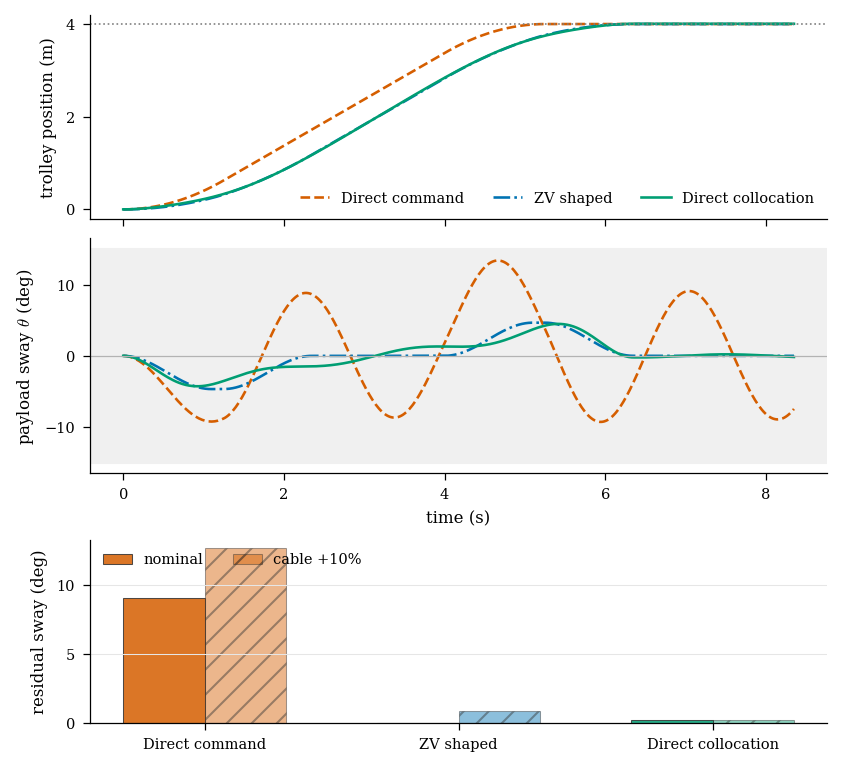
The ZV shaper produces the smallest nominal residual sway because the simulated plant closely matches the single oscillatory mode used to design it. The collocation command uses less squared acceleration than either baseline and keeps residual sway below one degree in both replays. The unshaped command completes the trolley move but leaves several degrees of oscillation. Cable-length mismatch increases the ZV residual substantially, while the collocation command degrades more gradually for this particular perturbation.
The table reports continuous-plant measurements rather than node values from the nonlinear program. Residual sway is the largest absolute angle after the common command horizon.
The animation uses the same high-accuracy nonlinear validation trajectories as the figure. It does not replay the collocation polynomial itself.
Figure 14:Continuous nonlinear replay of the unshaped, zero-vibration-shaped, and direct-collocation commands. All panels use the same spatial and temporal scales.
Inspect the direct-transcription implementation
1 2 3 4 5 6 7 8 9 10 11 12 13 14 15 16 17 18 19 20 21 22 23 24 25 26 27 28 29 30 31 32 33 34 35 36 37 38 39 40 41 42 43 44 45 46 47 48 49 50 51 52 53 54 55 56 57 58 59 60 61 62 63 64 65 66 67 68 69 70 71 72 73 74 75 76 77 78 79 80 81 82 83 84 85 86 87 88 89 90 91 92 93def solve_direct_collocation( params: CraneParameters | None = None, *, intervals: int = 28, horizon: float | None = None, max_iterations: int = 350, ) -> CollocationSolution: """Solve a constrained nonlinear point-to-point transcription. States and accelerations at every node are decision variables. Trapezoidal defects enforce the nonlinear dynamics, while boundary and path constraints are imposed directly on the node values. """ params = params or CraneParameters() params.validate() if intervals < 8: raise ValueError("intervals must be at least eight") move = TrapezoidalMove( params.target_position, params.profile_acceleration, params.profile_max_speed, ) shaper = ZeroVibrationShaper.from_parameters(params) if horizon is None: horizon = move.duration + shaper.delay if horizon <= 0.0: raise ValueError("horizon must be positive") node_time = np.linspace(0.0, horizon, intervals + 1) step = horizon / intervals state_guess, acceleration_guess = _initial_guess(params, node_time, move, shaper) initial = _pack(state_guess, acceleration_guess) initial_state = np.zeros(4) terminal_state = np.array([params.target_position, 0.0, 0.0, 0.0]) def objective(vector: np.ndarray) -> float: state, acceleration = _unpack(vector, intervals) return _transcription_objective(state, acceleration, step) def equality(vector: np.ndarray) -> np.ndarray: state, acceleration = _unpack(vector, intervals) defects = np.empty((intervals, 4)) for k in range(intervals): left = crane_dynamics(state[k], acceleration[k], params) right = crane_dynamics(state[k + 1], acceleration[k + 1], params) defects[k] = state[k + 1] - state[k] - 0.5 * step * (left + right) return np.concatenate( [state[0] - initial_state, defects.ravel(), state[-1] - terminal_state] ) nodes = intervals + 1 lower_state = np.tile( np.array([-0.25, -params.velocity_limit, -params.sway_limit, -2.0]), (nodes, 1), ) upper_state = np.tile( np.array( [params.target_position + 0.25, params.velocity_limit, params.sway_limit, 2.0] ), (nodes, 1), ) lower = _pack(lower_state, np.full(nodes, -params.acceleration_limit)) upper = _pack(upper_state, np.full(nodes, params.acceleration_limit)) result = minimize( objective, initial, method="SLSQP", bounds=list(zip(lower, upper)), constraints={"type": "eq", "fun": equality}, options={"maxiter": max_iterations, "ftol": 2e-10, "disp": False}, ) state, acceleration = _unpack(result.x, intervals) max_defect = float(np.max(np.abs(equality(result.x)))) success = bool(result.success and max_defect < 2e-5) if not success: raise RuntimeError( "crane direct collocation failed: " f"{result.message}; maximum equality residual {max_defect:.3e}" ) return CollocationSolution( time=node_time, state=state, acceleration=acceleration, objective=float(result.fun), max_defect=max_defect, success=success, message=str(result.message), )
Download the complete crane experiment
The optimization checks algebraic defects, bounds, and endpoint conditions at the nodes. The separate nonlinear replay checks what happens between those nodes. A small nodal defect is evidence that the discrete NLP was solved accurately; it is not, by itself, evidence that the mesh resolves the continuous dynamics.
The comparison does not establish that collocation always outperforms input shaping. The ZV calculation is inexpensive and can nearly cancel residual vibration when a lightly damped mode is accurately known. Direct collocation becomes useful when several state and actuator constraints must be handled together. All three commands remain open loop here. Feedback or receding-horizon replanning would be needed to react to unmeasured disturbances during the move.
Exercises
Lagrange interpolation practice
The worked example and first four exercises form a classroom sequence of about 30--40 minutes. They progress from constructing a polynomial through prescribed values to integrating a control on one physical time interval. The final exercise introduces barycentric evaluation as an optional extension. Each solution is collapsed so that the problems can be attempted first.
Worked example: recovering a quadratic
Suppose we know the values of only at and want a polynomial of degree at most two passing through them. These are physical coordinates for this example; they need not lie in the normalized interval . The nodes and values are
To attach a basis function to , put zeros at the other two nodes and normalize its value at . Repeat for the remaining nodes:
For example, at the three basis values are , so their weighted sum returns . At any other time, evaluate the same functions and combine them with the same stored values. Expanding gives
The reconstruction agrees with everywhere because itself is a polynomial of degree two. Three samples of a general function would determine its quadratic interpolant, but would not determine that function between samples. Here, for instance, has the same three sampled values and differs between them.
Solution to Exercise 2
The basis functions are and . Combining the stored values gives
Its Lagrange coefficients are , the endpoint values. Its monomial coefficients are , the intercept and slope. The polynomial has the same endpoint values because the added term vanishes at both endpoints. It is quadratic, so it lies outside the original degree restriction.
Solution to Exercise 3
Putting zeros at the other two nodes and normalizing at the selected node gives
The rows of their values at are , , and . Adding the expanded expressions cancels the quadratic and linear terms and leaves one. The interpolant is
At , the basis values are . They sum to one but include a negative weight. The interpolant therefore need not stay within the range of its nodal values.
Solution to Exercise 4
Only the coefficient of changes, so
The change at is , giving . The endpoints are unchanged because vanishes there.
For the original polynomial, vanishes at . Since , this point is its maximum, with
Changing a nodal decision variable changes the curve between nodes through its basis function. Likewise, bounds on the nodal variables alone do not ensure bounds on a quadratic state trajectory between nodes. The transcription needs additional checks there, as described in Checking the continuous trajectory.
Solution to Exercise 5
The only nonzero control value is at the midpoint, so . Integrating the expanded basis functions gives
Because , the displacement is . Integrating only as far as the current gives the state piece
It is cubic, with , as required. The endpoint constraint for arbitrary stored values is
For and the prescribed controls, it requires . This integration is exact for the chosen quadratic control and the dynamics ; no claim of exactness for general nonlinear dynamics is needed.
Solution to Exercise 6
The products of node differences give . At , the numerator and denominator are
Their ratio is , agreeing with . Multiplying every weight by the same nonzero number scales both sums equally and leaves their ratio unchanged. At a query that equals a node, return the stored value directly: . The polynomial is defined there, but the individual quotients in this evaluation formula divide by zero.
Further exercises
The following exercises revisit polynomial coordinates and connect them to the complete collocation schemes and trajectory checks developed in the chapter.
Solution to Exercise 7
Solution to Exercise 8
Problems 1 and 4 are interpolation problems; the least-squares formulation in problem 4 has a zero-residual interpolating solution. Problem 2 is regression. Problem 3 is neither statistical regression nor interpolation of observations: the unknown nodal values define an interpolating polynomial, and collocation adds equality constraints that select those values.
Solution to Exercise 9
Solution to Exercise 10
One node gives the constant derivative interpolant or . Integration yields the explicit or implicit Euler defect and a degree-one state. With endpoint nodes, . Its integral at is , which gives the trapezoidal defect. The linear derivative integrates to a degree-two state.
Solution to Exercise 11
Three distinct slope values define a quadratic derivative interpolant. Integrating that quadratic adds one degree, so the state is cubic. Integrating the cardinal functions over gives and hence the Simpson defect. Integrating to gives ; eliminating the midpoint slope with the endpoint defect gives
Solution to Exercise 12
The cardinal function is , so , , and . The stage equation gives , while the endpoint equation gives . Eliminating the slope between these equations gives and hence
The unknown right state appears inside the dynamics evaluation, which makes the rule implicit. The state polynomial is linear and the control constant. For the scalar problem with two half-unit intervals, the complete NLP is
The defects imply . Substitution into the objective gives , so both controls are one, , and the minimum cost is one. This recovers the opening trajectory on a finer mesh.
Solution to Exercise 13
Both controls are zero at both endpoints. The trapezoidal defect therefore predicts for either command. Their actual displacements are zero and
Endpoint samples cannot detect the quadratic control’s interior variation. Restricting the control to a line makes two zero endpoint values determine the zero control. Alternatively, a midpoint stage samples the second control at value one, so the two commands produce different stage slopes. With all three stages, Simpson weights integrate this quadratic control exactly.
Solution to Exercise 14
The NLP defect measures its equality constraints at the selected nodes. A coarse polynomial can satisfy those constraints while failing to resolve behavior between them. Evaluate and path constraints on the polynomial at additional times. Separately, integrate the original ODE using the chosen control and compare the simulated states with the polynomial. Refine the offending intervals or raise the local degree, then solve and validate again. Tightening an already small NLP tolerance does not fix representation error.
Summary and Outlook
Direct collocation turns an optimization over whole functions into an optimization over finitely many state and control values. These nodal values define polynomial segments. Algebraic defect constraints then require each segment to agree with the ODE at selected points.
Each polynomial has two equivalent descriptions: basis coefficients or values at nodes,
Direct collocation uses the nodal description because the stored values have an immediate physical meaning. Lagrange cardinal functions turn them into fixed operators for computing derivatives, endpoints, and integrals. Although this construction resembles polynomial fitting, the nodal values are optimization variables rather than noisy observations, and the ODE residual is an equality constraint rather than a regression loss.
Both integration and differentiation forms impose collocation at selected nodes. The integration form interpolates evaluated ODE slopes and uses state-matching residuals to make their integral agree with the stored states. The differentiation form interpolates state values and uses slope-matching residuals to make their derivative agree with the ODE. With matching node choices, degree, and control space, both describe the same feasible polynomial trajectories.
Interpolating one left or right slope gives explicit or implicit Euler and a linear state approximation. Interpolating both endpoint slopes gives the trapezoidal defect and a quadratic state approximation. Adding the midpoint slope gives Simpson weights, the Hermite--Simpson midpoint relation, and a cubic state approximation.
The control degree is chosen separately. Its support values determine the stage controls through the evaluation matrix . A program can construct , , and from the selected nodes, then assemble the same stage, endpoint, and cost expressions for all these schemes. Changing the nodes or control representation changes the finite approximation without requiring a new derivation of those expressions.
Across many intervals, each defect involves only neighboring endpoints and local stage values. Most entries in the constraint Jacobian are therefore zero, which allows an NLP solver to exploit a sparse, block-banded structure. The overhead-crane example also shows why solving the NLP is not the final check: constraints that hold at the nodes may still be violated between them. Polynomial residuals assess the local approximation, and independent simulation checks the trajectory produced by the chosen control.
How can we improve a control sequence when a simulator evaluates its cost but does not provide derivatives? Model Predictive Path Integral Control samples candidate control sequences and combines them using cost-dependent weights. When physical disturbances make the rollout uncertain, several simulated futures estimate each candidate’s expected cost. The following receding-horizon control chapter studies how replanning from measurements supplies feedback to a finite-horizon optimizer.
- Kelly, M. (2017). An Introduction to Trajectory Optimization: How to Do Your Own Direct Collocation. SIAM Review, 59(4), 849–904. 10.1137/16M1062569
- Andersson, J. A. E., Gillis, J., Horn, G., Rawlings, J. B., & Diehl, M. (2019). CasADi: A Software Framework for Nonlinear Optimization and Optimal Control. Mathematical Programming Computation, 11(1), 1–36. 10.1007/s12532-018-0139-4