The Pontryagin recursion exposes the temporal structure of first-order optimality, but a solver still needs a finite vector of variables and constraints. Should the states remain explicit, be eliminated by simulation, or appear only at selected segment boundaries?
Each choice recasts the discrete-time optimal control problem as a standard nonlinear program (NLP). Collect all decision variables (states, controls, and any auxiliary variables) into a single vector and write
with maps , , and . In optimal control, typically encodes dynamics and boundary conditions, while captures path and box constraints.
Thus uppercase stacks the inequalities , and uppercase stacks the equalities , following the conventions of the optimal-control formulation and the nonlinear-programming appendix.
There are multiple ways to arrive at (and benefit from) this NLP:
Simultaneous (direct transcription / full discretization): keep all states and controls as variables and impose the dynamics as equality constraints. This is straightforward and exposes sparsity, but the problem can be large unless solver-side techniques (e.g., condensing) are exploited.
Sequential (recursive elimination / single shooting): eliminate states by forward propagation from the initial condition, leaving controls as the main decision variables. This reduces dimension and constraints, but can be sensitive to initialization and longer horizons.
Multiple shooting: introduce state variables at segment boundaries and enforce continuity between simulated segments. This compromises between size and conditioning and is often more robust than pure single shooting.
Learning Goals
After working through the examples and exercises, you should be able to:
Formulate simultaneous, single-shooting, and multiple-shooting programs.
Compare their variables, constraints, sparsity, and sensitivity paths.
Differentiate a rollout in reverse mode to measure how each control affects the terminal state, and relate that sensitivity to the conditioning of a shooting program.
Construct continuity defects between independently simulated segments and check a computed trajectory against its dynamics and constraints.
Prerequisites
The formulations use the finite-horizon optimal-control problem and its Pontryagin recursion. The nonlinear-programming appendix reviews constrained optimization, derivatives, and numerical solvers.
Simultaneous Methods
What numerical structure appears when every state and action remains an optimization variable and each transition becomes an equality constraint?
In the simultaneous (also called direct transcription or full discretization) approach, we keep the entire trajectory explicit and enforce the dynamics as equality constraints. Starting from the Bolza DOCP,
collect all variables into a single vector
The dynamics residual is written here as . Its multiplier is the negative of the Pontryagin costate, which multiplies ; reversing an equality residual changes its multiplier sign but leaves the feasible trajectories unchanged.
Path constraints typically apply only at selected times. Let index additional equality constraints and index inequality constraints . For each constraint , define the set of time indices where it is enforced (e.g., terminal constraints use ). The simultaneous transcription is the NLP
optionally with simple bounds and folded into or provided to the solver separately. For notational convenience, some constraints may not depend on at times in ; the indexing still helps specify when each condition is active.
This direct transcription is attractive because it is faithful to the model and exposes sparsity. The Jacobian of has a block bi-diagonal structure induced by the dynamics, and the KKT matrix is sparse and structured. These properties are exploited by interior-point and SQP methods. The trade-off is size: with state dimension and control dimension , the decision vector has entries, and there are roughly dynamic equalities plus any path and boundary conditions. Techniques such as partial or full condensing eliminate state variables to reduce the equality set (at the cost of denser matrices), while keeping states explicit preserves sparsity and often improves robustness on long horizons and in the presence of state constraints.
Compared to alternatives, simultaneous methods avoid the long nonlinear dependency chains of single shooting and make it easier to impose state/path constraints. They can, however, demand more memory and per-iteration linear algebra, so practical performance hinges on exploiting sparsity and good initialization.
The same logic applies when selecting an optimizer. For small-scale problems, it is common to rely on general-purpose routines such as those in scipy.optimize.minimize. Derivative-free methods like Nelder–Mead require no gradients but scale poorly as dimensionality increases. Quasi-Newton schemes such as BFGS work well for moderate dimensions and can approximate gradients by finite differences, while large-scale trajectory optimization often calls for gradient-based constrained solvers such as interior-point or sequential quadratic programming methods that can exploit sparse Jacobians and benefit from automatic differentiation. Stochastic techniques, including genetic algorithms, simulated annealing, or particle swarm optimization, occasionally appear when gradients are unavailable, but their cost grows rapidly with dimension and they are rarely competitive for structured optimal control problems.
Example: Nonlinear Cart-Pole Swing-Up
A cart carries a rigid pendulum whose angle is measured from the upright vertical. The cart can accelerate horizontally, but no actuator applies torque directly at the pendulum joint. Starting from the stable downward configuration, the task is to move the base so that the pendulum arrives upright while the cart returns near the center of a finite rail.
Let the state be , where and are the cart position and velocity, and and are the pendulum angle and angular velocity. A commanded horizontal acceleration produces the nonlinear dynamics
The factor identifies the action channel. Horizontal base motion couples into angular acceleration, and its sign and magnitude depend on the current configuration. A black-box optimizer could evaluate these equations without inspecting that term, but the term explains why the cart must first move away from its eventual resting position to build pendulum energy.
The numerical experiment uses a 4.5 s horizon with zero-order-hold controls and a step size s. Fourth-order Runge--Kutta integration defines the discrete map . Both numerical formulations solve the same problem:
The periodic penalty assigns the same terminal cost to angles that differ by a full revolution. Position and velocity penalties still require the cart to finish near rest, so rotating the pole through the top is not enough by itself.
Direct transcription retains all 31 states and 30 controls. It therefore optimizes over 154 scalar variables and imposes 124 scalar equalities, including the initial condition and one four-dimensional dynamics equation per step. The equality Jacobian is block banded because the residual at step depends only on .
The small demonstration below passes that Jacobian to SLSQP as a dense array. A large-scale direct solver would instead store and factor the same block-banded pattern sparsely. The formulation exposes sparsity, but exploiting it is a separate implementation choice.
Sequential Methods
Can eliminating the states reduce the nonlinear program without making the resulting long simulation chain too sensitive to early actions?
The previous section showed how a discrete-time optimal control problem can be solved by treating all states and controls as decision variables and enforcing the dynamics as equality constraints. This produces a nonlinear program that can be passed to solvers such as scipy.optimize.minimize with the SLSQP method. For short horizons, this approach is straightforward and works well; the code stays close to the mathematical formulation.
It also has a real advantage: by keeping the states explicit and imposing the dynamics through constraints, we anchor the trajectory at multiple points. This extra structure helps stabilize the optimization, especially for long horizons where small deviations in early steps can otherwise propagate and cause the optimizer to drift or diverge. In that sense, this formulation is better conditioned and more robust than approaches that treat the dynamics implicitly.
The drawback is scale. As the horizon grows, the number of variables and constraints grows with it, and all are coupled by the dynamics. Each iteration of a sequential quadratic programming (SQP) or interior-point method requires building and factorizing large Jacobians and Hessians. These methods have been embedded in reinforcement learning and differentiable programming pipelines, through implicit layers or differentiable convex solvers, but the cost is significant. They remain serial, rely on repeated linear algebra factorizations, and are difficult to parallelize efficiently. When thousands of such problems must be solved inside a learning loop, the overhead becomes prohibitive.
This motivates an alternative that aligns with the computational model of machine learning. For deterministic dynamics, the equality constraints can be eliminated by making the states implicit. Instead of solving for both states and controls, we fix the initial state and roll the system forward under a candidate control sequence. State constraints can remain, but they become nonlinear functions of the entire preceding control sequence. This is the essence of single shooting.
The term “shooting” comes from the idea of aiming and firing a trajectory from the initial state: you pick a control sequence, integrate (or step) the system forward, and see where it lands. If the final state misses the target, you adjust the controls and try again: like adjusting the angle of a shot until it hits the mark. It is called single shooting because we compute the entire trajectory in one pass from the starting point, without breaking it into segments. Later, we will contrast this with multiple shooting, where the horizon is divided into smaller arcs that are optimized jointly to improve stability and conditioning.
The analogy with deep learning is also immediate: the control sequence plays the role of parameters, the rollout is a forward pass, and the cost is a scalar loss. Gradients can be obtained with reverse-mode automatic differentiation. In the single shooting formulation of the DOCP, the constrained program
collapses to
Here denotes the state reached at time by recursively applying the dynamics to the previous state and current control. This recursion can be written as
Concretely, here is JAX-style pseudocode for defining phi(u, x_0, t) using jax.lax.scan with a zero-based time index:
def phi(u_seq, x0, t):
    """Return \phi_t(u, x0) with 0-based t (\phi_0 = x0).

    u_seq: controls of length T (or T-1); only first t entries are used
    x0: initial state at time 0
    t: integer >= 0
    """
    if t <= 0:
        return x0

    def step(carry, u):
        x, t_idx = carry
        x_next = f(x, u, t_idx)
        return (x_next, t_idx + 1), None

    (x_t, _), _ = lax.scan(step, (x0, 0), u_seq[:t])
    return x_t
The pattern mirrors an RNN unroll: starting from an initial state () and a sequence of controls (), we propagate forward through the dynamics, updating the state at each step and accumulating cost along the way. This structural similarity is why single shooting often feels natural to practitioners with a deep learning background: the rollout is a forward pass, and gradients propagate backward through time exactly as in backpropagation through an RNN.
Algorithmically:
In JAX or PyTorch, this loop can be compiled and differentiated automatically. The control sequence plays the role of trainable parameters, while the simulated trajectory is the forward computation. Reverse-mode differentiation of that computation gives .
Single shooting is attractive for its simplicity and compatibility with differentiable programming, but it has limitations. Early controls influence every later state through a long product of dynamics Jacobians. This can make gradients poorly conditioned over long horizons. State constraints also lose their local sparse representation because each constrained state depends on all earlier controls. Formulations that keep selected states explicit, such as multiple shooting or collocation, shorten these dependency chains.
Matched Swing-Up Comparison
The direct-transcription and single-shooting implementations below use the cart-pole problem stated above without changing the model, cost, limits, horizon, initial control guess, or nonlinear-programming solver. Only the decision variables and the representation of the dynamics differ.
Figure 1:Direct transcription and single shooting solve the same nonlinear cart-pole problem from the same initialization. Both reach the upright configuration and respect the matched limits, but they converge to different local solutions. Direct transcription retains 154 scalar variables and 124 local dynamics equalities; single shooting retains only the 30 controls and reconstructs every state by forward simulation.
method                variables  eqs  iterations  objective  final angle  defect
direct transcription    154  124         413      1.180      0.002 deg  1.3e-07
single shooting          30    0         430      2.675      0.130 deg  0.0e+00
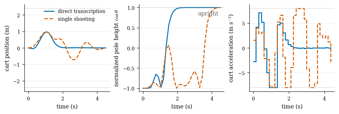
Both solvers produce a successful open-loop swing-up. The direct formulation reaches a lower objective in this fixed run, while single shooting uses a much smaller decision vector. This numerical outcome does not establish that direct transcription always finds better solutions. It exposes a concrete trade-off: eliminating variables shortens the program but lengthens the dependency from an early control to the terminal cost and later constraints.
Figure 2:The two trajectories are generated by the same nonlinear RK4 plant. The pole starts downward and reaches the upright configuration while the cart remains inside the 2.4 m rail limits. Animation frames are computed from the optimized state trajectories; no browser-side simulator is used.
The comparison also separates optimization from feedback. Each optimizer returns one fixed control sequence for one assumed initial state. To test what that object can and cannot do, the next replay applies the direct-transcription controls twice. One realization follows the nominal model. The other receives an additional cart acceleration of for one 0.15 s step at s, after which both realizations receive the same remaining commands.
Figure 3:A one-step unmodeled acceleration separates two realizations driven by the same open-loop controls. The nominal trajectory reaches normalized pole height ; the disturbed trajectory finishes below the horizontal. The optimizer has produced a plan, not a rule that reacts to the observed state.
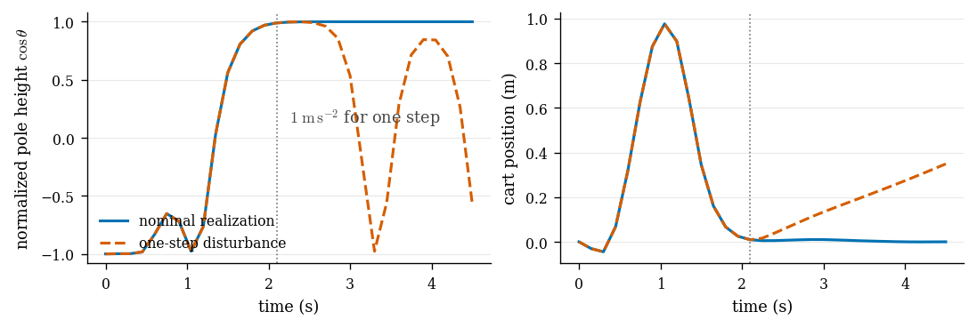
Feedback changes the object being computed. A feedback controller maps the state observed after the disturbance to a new action. Model predictive control will obtain such a map by repeatedly solving trajectory problems, while dynamic programming will construct state-contingent decisions through the value function.
Inspect the shared nonlinear dynamics
1 2 3 4 5 6 7 8 9 10 11 12 13 14 15 16 17 18def cartpole_dynamics( state: np.ndarray, acceleration: float, parameters: CartPoleParameters = CartPoleParameters(), ) -> np.ndarray: """Continuous nonlinear dynamics with angle measured from upright.""" position, velocity, angle, angular_velocity = np.asarray(state, dtype=float) del position angular_acceleration = ( parameters.gravity * np.sin(angle) - acceleration * np.cos(angle) ) / parameters.pole_length - parameters.angular_damping * angular_velocity return np.array( [velocity, acceleration, angular_velocity, angular_acceleration], dtype=float, )
Download the complete cart-pole trajectory-optimization and control source.
Example: Alley-Docking a Semi Truck
The cart-pole comparison kept the solver fixed and changed the decision variables. This example stays with single shooting and asks what its one long rollout does to the derivatives the optimizer receives. A tractor-semitrailer backing into a loading bay is a useful test because the rig has a well-known instability: in reverse, a small steering error grows into a jackknife unless it is corrected. That growth is the long product of dynamics Jacobians mentioned above, and it can be measured on the solution.
The model. The state is the tractor’s rear-axle position , the tractor heading , and the trailer heading . The fifth wheel sits over the tractor’s rear axle, and the trailer axle trails it by along the trailer axis. The controls are the tractor speed and the steering angle , which act through the kinematic model
with tractor wheelbase . The hitch angle is zero when the rig is straight. The controls are held constant over intervals of , each integrated with one RK4 step, and intervals cover a fixed maneuver. Speed is bounded by and steering by .
The maneuver. The dock face is the line and the bay is centered on . The rig starts in a lane parallel to the dock, out, pointing along with the trailer behind it. It must end straight and pointing away from the dock, with the trailer’s rear bumper from the face. A second scenario exchanges the endpoints: the rig starts docked and must pull out to the lane position.
The program. Single shooting keeps only the control values as decision variables. The objective is the cost of the rollout they generate,
The stage cost charges speed, steering, and the distance between the trailer axle and its target, and adds two smooth penalties evaluated on the rolled-out state: one for any body corner closer than to the dock face and one for hitch angles beyond . These are state constraints of the kind discussed above, and in this formulation each one becomes a function of every earlier control. The term depends on the controls alone. It charges changes between consecutive intervals and a moving final interval. The terminal cost penalizes the trailer-axle position error, the trailer heading error, and the hitch angle. The control bounds stay explicit and are handled by the solver.
The implementation follows Algorithm 1. A
jax.lax.scan rollout produces the states, the cost is accumulated along
it, and jax.value_and_grad returns with its gradient by
reverse mode. SciPy’s L-BFGS-B receives both, together with the box on each
control, and stops when the projected gradient falls below 10-5 or the
relative decrease of falls below 10-10. The seed is a straight creep
at in the relevant direction: backing for the docking
scenario and forward for the pull-out.
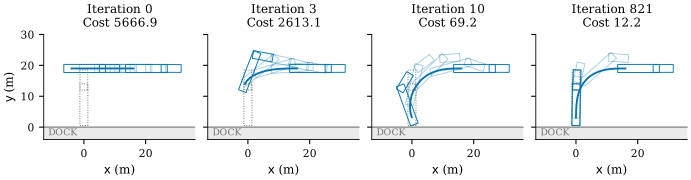
Figure 4:Four L-BFGS-B iterates of the backing solve. Each panel is a complete rollout of the current control sequence, with the trailer-axle path in blue and rig outlines every ten seconds; the dotted outline is the target. The seed backs straight along the lane. By iteration 10 the trailer swings toward the bay, and the final plan docks it.
Figure 5:Final plans for both scenarios. The blue curve is the trailer axle, the dashed orange curve the tractor axle, and the dotted gray line the straight seed. Outlines show the rig every five seconds. In the online book this figure is a replay: choose a scenario and an optimizer checkpoint, then scrub or play simulation time within that fixed plan. The path ahead and the translucent outlines show the plan’s remaining states; the tiles and plots belong to the selected checkpoint, including early ones that do not dock.
| Scenario | Stop | Iterations | Objective evaluations | Initial cost | Final cost |
|---|---|---|---|---|---|
| Backing into the bay | small decrease | 821 | 1750 | 5666.9 | 12.2009 |
| Pulling out of the bay | small decrease | 510 | 1044 | 5666.9 | 11.3762 |
The arrival checks below use the finer replay.
| Scenario | Trailer-axle error (m) | Trailer heading error (°) | Hitch angle (°) | Clearance (m) | Largest hitch angle (°) | Distance (m) |
|---|---|---|---|---|---|---|
| Backing into the bay | 0.0031 | 0.872 | 1.72 | 0.466 | 45.4 | 32.2 |
| Pulling out of the bay | 0.00205 | 0.599 | 1.3 | 0.500 | 42.5 | 36.1 |
Amplification of a steering perturbation into the terminal hitch angle, at the first control interval of each plan.
| Plan | Reverse mode | Per-interval product |
|---|---|---|
| Backing into the bay | 14.2 | 14.2 |
| Pulling out of the bay | 0.0737 | 0.0737 |
| Backing plan driven forward | 0.0695 | 0.0695 |
Both solves stop on a small relative decrease of the objective and pass the arrival checks, which replay the final controls with four RK4 substeps per interval. Backing needed 821 iterations and 1750 objective evaluations, pulling out 510 and 1044. The docking plan backs at the speed limit for the first 17 seconds. Its steering starts at , which bends the rig, sweeps through zero, and reaches at 17 seconds as the trailer swings toward the bay; speed and steering then relax together as the rig straightens. The hitch angle peaks near , inside the limit (Figure 6). The pull-out plan overshoots the lane position slightly and backs up to straighten the rig, which is why its distance is longer.
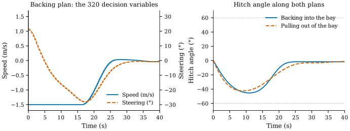
Figure 6:Left: the final backing plan, that is, the 320 numbers the optimizer returns. Speed saturates at the reverse limit and steering approaches its limit before both relax as the rig straightens. Right: the hitch angle along both final plans; dotted lines mark the penalty threshold.
Measuring the sensitivity chain. Subtracting the two heading equations gives a closed equation for the hitch angle,
Along a given plan, a small hitch perturbation evolves as . Driving forward, , the coefficient is negative and the perturbation decays. Backing, , it is positive and the perturbation grows: this is the jackknife instability. Over one control interval of length the perturbation is multiplied by , and the effect of a steering change at interval on the terminal hitch angle is the product of these factors over all later intervals. For a straight rig the product is , where is the distance still to be backed after interval : every ten metres of backing multiplies an uncorrected hitch error by .
This product is what reverse-mode differentiation computes through the
rollout. Figure 7 compares the two. The dots are
from jax.jacrev, divided by the tractor
heading change that the same steering causes within interval , so that a
value of one means the rest of the rollout neither amplifies nor attenuates
the error. The lines are the products of per-interval factors along the same
plan. They agree to within half a percent. For the backing plan, a steering
error at the start of the maneuver is amplified fourteen times by the time
the trailer reaches the dock. For the same path driven forward, obtained by
reversing the control sequence and the sign of the speed, an early steering
error is attenuated to 0.07 of its immediate effect, because the trailer
follows the tractor and forgets.
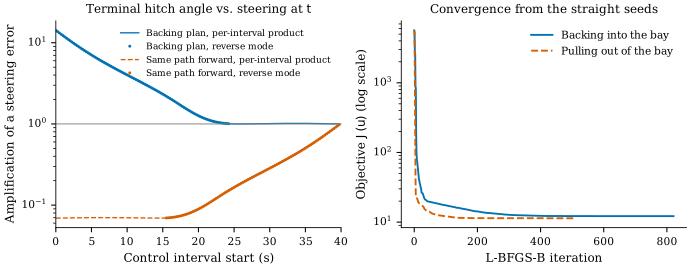
Figure 7:Left: amplification of a steering perturbation into the terminal hitch angle, per control interval, for the final backing plan and for the same path driven forward. Dots come from reverse-mode differentiation of the rollout; lines are products of the linearized per-interval hitch Jacobians. Intervals with speed below are omitted because a stationary tractor cannot steer. Right: objective value at every L-BFGS-B iteration for the two scenarios, which start from the same seed cost.
The consequence for the optimizer appears in the right panel. At the seed, the gradient of with respect to the first steering angle is about 800 in the backing scenario and about 200 in the pull-out, while the gradient with respect to the last steering angle is 0.04 in both. The curvature of varies across the decision vector in the same way, more strongly for backing. The backing solve descends more slowly, stops later, and ends with a projected gradient roughly three times larger than the pull-out solve. Two local solves do not establish a general rule, but they show the mechanism: eliminating the states did not remove the dynamics from the problem, it moved them into the derivatives. A longer backing distance multiplies the amplification by every ten metres, and the formulation of the next section shortens that chain by keeping selected states as variables.
Inspect the reduced objective and the L-BFGS-B driver
1 2 3 4 5 6 7 8 9 10 11 12 13 14 15 16 17 18 19 20 21 22 23 24 25 26 27 28 29 30 31 32 33 34 35 36 37 38 39 40 41 42 43 44 45 46 47 48 49 50 51 52 53 54 55 56 57 58 59 60 61 62 63 64 65 66 67 68 69 70 71 72 73 74 75 76 77 78 79 80 81 82 83 84 85 86 87 88 89 90 91 92 93 94 95 96 97 98 99 100 101 102 103 104 105 106 107 108 109 110 111 112 113 114 115 116 117 118 119 120 121 122 123 124 125 126 127 128 129 130 131 132 133 134def shooting_objective(controls, initial, goal, parameters=TruckParameters()): """The reduced objective J(u): roll the plan out from x_0, then price it.""" states = rollout(initial, controls, parameters) return total_cost(states, controls, goal, parameters) def control_bounds(parameters=TruckParameters()): lower = np.tile([-parameters.speed_limit, -parameters.steering_limit], parameters.steps) return lower, -lower def initial_controls(parameters=TruckParameters(), speed=-0.5): """Creep straight at a constant speed: a plausible seed, not a solution.""" return np.tile([speed, 0.], (parameters.steps, 1)) def checkpoint_schedule(max_iterations, dense=10, factor=1.2): """Iterations whose full plans are kept: every early one, then geometrically spaced.""" kept, value = set(range(dense + 1)), float(dense) while value < max_iterations: value *= factor kept.add(int(round(value))) kept.add(max_iterations) return kept @dataclass class ShootingResult: states: np.ndarray controls: np.ndarray history: list cost_trace: np.ndarray status: str iterations: int objective_evaluations: int projected_gradient: float solver_seconds: float @property def converged(self): return self.status == "converged" def _projected_gradient(controls, gradient, lower, upper): return float(np.max(np.abs(controls - np.clip(controls - gradient, lower, upper)))) def solve_single_shooting(initial, goal, seed, parameters=TruckParameters(), max_iterations=1500, gradient_tolerance=1e-5, relative_tolerance=1e-10, checkpoints=None): """Minimize J(u) over the control sequence alone with L-BFGS-B. The objective and its reverse-mode gradient come from one compiled rollout. SciPy's bound-constrained L-BFGS-B handles the control box and stops on the projected gradient or on a small relative decrease. The cost of every iterate is kept; complete plans are kept at the checkpoint iterations and at the end. """ p = parameters initial, goal, seed = (np.asarray(v, float) for v in (initial, goal, seed)) if initial.shape != (4,) or goal.shape != (4,) or seed.shape != (p.steps, 2): raise ValueError("states need four entries and the seed needs steps x 2 controls") lower, upper = control_bounds(p) if np.any(seed.ravel() < lower) or np.any(seed.ravel() > upper): raise ValueError("initial controls must respect their bounds") if max_iterations < 0: raise ValueError("invalid iteration budget") checkpoints = checkpoint_schedule(max_iterations) if checkpoints is None else set(checkpoints) x0, target = jnp.asarray(initial), jnp.asarray(goal) @jax.jit def value_and_gradient(flat): controls = flat.reshape(p.steps, 2) value, gradient = jax.value_and_grad( lambda u: shooting_objective(u, x0, target, p))(controls) return value, gradient.ravel() roll = jax.jit(lambda flat: rollout(x0, flat.reshape(p.steps, 2), p)) evaluations = 0 def evaluate(flat): nonlocal evaluations evaluations += 1 value, gradient = value_and_gradient(jnp.asarray(flat)) return float(value), np.asarray(gradient) # Compile before timing. value_and_gradient(jnp.asarray(seed.ravel())) roll(jnp.asarray(seed.ravel())) history, cost_trace = [], [] def record(iteration, flat, force=False): value, gradient = evaluate(flat) cost_trace.append(value) if force or iteration in checkpoints: history.append(dict( iteration=iteration, cost=value, states=np.asarray(roll(jnp.asarray(flat))), controls=np.asarray(flat).reshape(p.steps, 2).copy(), projected_gradient=_projected_gradient(flat, gradient, lower, upper))) count = 0 def callback(flat): nonlocal count count += 1 record(count, flat) started = perf_counter() record(0, seed.ravel(), force=True) outcome = minimize(evaluate, seed.ravel(), jac=True, method="L-BFGS-B", bounds=list(zip(lower, upper)), callback=callback, options={"maxiter": max_iterations, "gtol": gradient_tolerance, "ftol": relative_tolerance, "maxcor": 30, "maxfun": 20 * max_iterations}) elapsed = perf_counter() - started final, iterations = np.asarray(outcome.x), int(outcome.nit) if history[-1]["iteration"] != iterations: record(iterations, final, force=True) cost_trace.pop() norm = history[-1]["projected_gradient"] if not np.all(np.isfinite(final)): status = "nonfinite" elif norm <= gradient_tolerance: status = "converged" elif iterations >= max_iterations: status = "iteration_limit" elif outcome.success: status = "small_decrease" else: status = "stalled" return ShootingResult(np.asarray(roll(jnp.asarray(final))), final.reshape(p.steps, 2), history, np.asarray(cost_trace), status, iterations, evaluations, float(norm), elapsed)
Run uv run python scripts/build_truck_parking_artifacts.py from the
repository root to reproduce the solves, figures, tables, and replay data.
Normal book builds read those artifacts.
In Between Sequential and Simultaneous
Can selected boundary states shorten those sensitivity paths while preserving local simulation inside each segment?
The two formulations we have seen so far lie at opposite ends. The full discretization approach keeps every state explicit and enforces the dynamics through equality constraints, which makes the structure clear but leads to a large optimization problem. At the other end, single shooting removes these constraints by simulating forward from the initial state, leaving only the controls as decision variables. That makes the problem smaller, but it also introduces a long and highly nonlinear dependency from the first control to the last state.
Multiple shooting sits in between. Instead of simulating the entire horizon in one shot, we divide it into smaller segments. For each segment, we keep its starting state as a decision variable and propagate forward using the dynamics for that segment. At the end, we enforce continuity by requiring that the simulated end state of one segment matches the decision variable for the next.
Formally, suppose the horizon of steps is divided into segments of length (with for simplicity). We introduce:
The controls for each step: .
The state at the start of each segment: .
Given and the controls in its segment, we compute the predicted terminal state by simulating forward:
where represents applications of the dynamics. Continuity constraints enforce:
The resulting nonlinear program looks like this:
Compared to the full NLP, we no longer introduce every intermediate state as a variable, only the anchors at segment boundaries. Inside each segment, states are reconstructed by simulation. Compared to single shooting, these anchors break the long dependency chain that makes optimization unstable: gradients only have to travel across steps before they hit a decision variable, rather than the entire horizon. This is the same reason why exploding or vanishing gradients appear in deep recurrent networks: when the chain is too long, information either dies out or blows up. Multiple shooting shortens the chain and improves conditioning.
By adjusting the number of segments , we can interpolate between the two extremes: gives single shooting, while recovers the full direct NLP. In practice, a moderate number of segments often strikes a good balance between robustness and complexity.
Source
#  label: fig-ocp-multiple-shooting
#  caption: Multiple shooting ballistic BVP: the code produces an animation (and optional static plot) that shows how segment defects shrink while steering the projectile to the target.

%config InlineBackend.figure_format = 'retina'
"""
Multiple Shooting as a Boundary-Value Problem (BVP) for a Ballistic Trajectory
-----------------------------------------------------------------------------
We solve for the initial velocities (and total flight time) so that the terminal
position hits a target, enforcing continuity between shooting segments.
"""

import numpy as np
import matplotlib.pyplot as plt

# Apply book style
try:
    import scienceplots
    plt.style.use(['science', 'notebook'])
except (ImportError, OSError):
    pass  # Use matplotlib defaults
from scipy.integrate import solve_ivp
from scipy.optimize import minimize
from IPython.display import HTML, display

# -----------------------------
# Physical parameters
# -----------------------------
g = 9.81          # gravity (m/s^2)
m = 1.0           # mass (kg)
drag_coeff = 0.1  # quadratic drag coefficient


def dynamics(t, state):
    """Ballistic dynamics with quadratic drag. state = [x, y, vx, vy]."""
    x, y, vx, vy = state
    v = np.hypot(vx, vy)
    drag_x = -drag_coeff * v * vx / m if v > 0 else 0.0
    drag_y = -drag_coeff * v * vy / m if v > 0 else 0.0
    dx  = vx
    dy  = vy
    dvx = drag_x
    dvy = drag_y - g
    return np.array([dx, dy, dvx, dvy])


def flow(y0, h):
    """One-segment flow map Φ(y0; h): integrate dynamics over duration h."""
    sol = solve_ivp(dynamics, (0.0, h), y0, method="RK45", rtol=1e-7, atol=1e-9)
    return sol.y[:, -1], sol

# -----------------------------
# Multiple-shooting BVP residuals
# -----------------------------

def residuals(z, K, x_init, x_target):
    """
    Unknowns z = [vx0, vy0, H, y1(4), y2(4), ..., y_{K-1}(4)]  (total len = 3 + 4*(K-1))
    We define y0 from x_init and (vx0, vy0). Each segment has duration h = H/K.
    Residual vector stacks:
      - initial position constraints: y0[:2] - x_init[:2]
      - continuity: y_{k+1} - Φ(y_k; h) for k=0..K-2
      - terminal position constraint at end of last segment: Φ(y_{K-1}; h)[:2] - x_target[:2]
    """
    n = 4
    vx0, vy0, H = z[0], z[1], z[2]
    if H <= 0:
        # Strongly penalize nonpositive durations to keep solver away
        return 1e6 * np.ones(2 + 4*(K-1) + 2)

    h = H / K

    # Build list of segment initial states y_0..y_{K-1}
    ys = []
    y0 = np.array([x_init[0], x_init[1], vx0, vy0], dtype=float)
    ys.append(y0)
    if K > 1:
        rest = z[3:]
        y_internals = rest.reshape(K-1, n)
        ys.extend(list(y_internals))  # y1..y_{K-1}

    res = []

    # Initial position must match exactly
    res.extend(ys[0][:2] - x_init[:2])

    # Continuity across segments
    for k in range(K-1):
        yk = ys[k]
        yk1_pred, _ = flow(yk, h)
        res.extend(ys[k+1] - yk1_pred)

    # Terminal position at the end of last segment equals target
    y_last_end, _ = flow(ys[-1], h)
    res.extend(y_last_end[:2] - x_target[:2])

    # Optional soft "stay above ground" at knots (kept gentle)
    # res.extend(np.minimum(0.0, np.array([y[1] for y in ys])).ravel())

    return np.asarray(res)

# -----------------------------
# Solve BVP via optimization on 0.5*||residuals||^2
# -----------------------------

def solve_bvp_multiple_shooting(K=5, x_init=np.array([0., 0.]), x_target=np.array([10., 0.])):
    """
    K: number of shooting segments.
    x_init: initial position (x0, y0). Initial velocities are unknown.
    x_target: desired terminal position (xT, yT) at time H (unknown).
    """
    # Heuristic initial guesses:
    dx = x_target[0] - x_init[0]
    dy = x_target[1] - x_init[1]
    H0 = max(0.5, dx / 5.0)  # guess ~ 5 m/s horizontal
    vx0_0 = dx / H0
    vy0_0 = (dy + 0.5 * g * H0**2) / H0  # vacuum guess

    # Intentionally disconnected internal knots to visualize defect shrinkage
    internals = []
    for k in range(1, K):  # y1..y_{K-1}
        xk = x_init[0] + (dx * k) / K
        yk = x_init[1] + (dy * k) / K + 2.0  # offset to create mismatch
        internals.append(np.array([xk, yk, 0.0, 0.0]))
    internals = np.array(internals) if K > 1 else np.array([])

    z0 = np.concatenate(([vx0_0, vy0_0, H0], internals.ravel()))

    # Variable bounds: H > 0, keep velocities within a reasonable range
    # Use wide bounds to let the solver work; tune if needed.
    lb = np.full_like(z0, -np.inf, dtype=float)
    ub = np.full_like(z0,  np.inf, dtype=float)
    lb[2] = 1e-2  # H lower bound
    # Optional velocity bounds
    lb[0], ub[0] = -50.0, 50.0
    lb[1], ub[1] = -50.0, 50.0

    # Objective and callback for L-BFGS-B
    def objective(z):
        r = residuals(z, K,
                      np.array([x_init[0], x_init[1], 0., 0.]),
                      np.array([x_target[0], x_target[1], 0., 0.]))
        return 0.5 * np.dot(r, r)

    iterate_history = []
    def cb(z):
        iterate_history.append(z.copy())

    bounds = list(zip(lb.tolist(), ub.tolist()))
    sol = minimize(objective, z0, method='L-BFGS-B', bounds=bounds,
                   callback=cb, options={'maxiter': 300, 'ftol': 1e-12})

    return sol, iterate_history

# -----------------------------
# Reconstruct and plot (optional static figure)
# -----------------------------

def reconstruct_and_plot(sol, K, x_init, x_target):
    n = 4
    vx0, vy0, H = sol.x[0], sol.x[1], sol.x[2]
    h = H / K

    ys = []
    y0 = np.array([x_init[0], x_init[1], vx0, vy0])
    ys.append(y0)
    if K > 1:
        internals = sol.x[3:].reshape(K-1, n)
        ys.extend(list(internals))

    # Integrate each segment and stitch
    traj_x, traj_y = [], []
    for k in range(K):
        yk = ys[k]
        yend, seg = flow(yk, h)
        traj_x.extend(seg.y[0, :].tolist() if k == 0 else seg.y[0, 1:].tolist())
        traj_y.extend(seg.y[1, :].tolist() if k == 0 else seg.y[1, 1:].tolist())

    # Plot
    fig, ax = plt.subplots(figsize=(7, 4.2))
    ax.plot(traj_x, traj_y, '-', label='Multiple-shooting solution')
    ax.plot([x_init[0]], [x_init[1]], 'go', label='Start')
    ax.plot([x_target[0]], [x_target[1]], 'r*', ms=12, label='Target')
    total_pts = len(traj_x)
    for k in range(1, K):
        idx = int(k * total_pts / K)
        ax.axvline(traj_x[idx], color='k', ls='--', alpha=0.3, lw=1)

    ax.set_xlabel('x (m)')
    ax.set_ylabel('y (m)')
    ax.set_title(f'Multiple Shooting BVP (K={K})   H={H:.3f}s   v0=({vx0:.2f},{vy0:.2f}) m/s')
    ax.grid(True, alpha=0.3)
    ax.legend(loc='best')
    plt.tight_layout()

    # Report residual norms
    res = residuals(sol.x, K, np.array([x_init[0], x_init[1], 0., 0.]), np.array([x_target[0], x_target[1], 0., 0.]))
    print(f"\nFinal residual norm: {np.linalg.norm(res):.3e}")
    print(f"vx0={vx0:.4f} m/s, vy0={vy0:.4f} m/s, H={H:.4f} s")

# -----------------------------
# Create JS animation for notebooks
# -----------------------------

def create_animation_progress(iter_history, K, x_init, x_target):
    """Return a JS animation (to_jshtml) showing defect shrinkage across segments."""
    import matplotlib.pyplot as plt
    from matplotlib.animation import FuncAnimation

    # Apply book style
    try:
        import scienceplots
        plt.style.use(['science', 'notebook'])
    except (ImportError, OSError):
        pass  # Use matplotlib defaults

    n = 4

    def unpack(z):
        vx0, vy0, H = z[0], z[1], z[2]
        ys = [np.array([x_init[0], x_init[1], vx0, vy0])]
        if K > 1 and len(z) > 3:
            internals = z[3:].reshape(K-1, n)
            ys.extend(list(internals))
        return H, ys

    fig, ax = plt.subplots(figsize=(7, 4.2))
    ax.set_xlabel('Segment index (normalized time)')
    ax.set_ylabel('y (m)')
    ax.set_title('Multiple Shooting: Defect Shrinkage (Fixed Boundaries)')
    ax.grid(True, alpha=0.3)

    # Start/target markers at fixed indices
    ax.plot([0], [x_init[1]], 'go', label='Start')
    ax.plot([K], [x_target[1]], 'r*', ms=12, label='Target')
    # Vertical dashed lines at boundaries
    for k in range(1, K):
        ax.axvline(k, color='k', ls='--', alpha=0.35, lw=1)
    ax.legend(loc='best')

    # Pre-create line artists
    colors = plt.cm.plasma(np.linspace(0, 1, K))
    segment_lines = [ax.plot([], [], '-', color=colors[k], lw=2, alpha=0.9)[0] for k in range(K)]
    connector_lines = [ax.plot([], [], 'r-', lw=1.4, alpha=0.75)[0] for _ in range(K-1)]

    text_iter = ax.text(0.02, 0.98, '', transform=ax.transAxes,
                        va='top', fontsize=9,
                        bbox=dict(boxstyle='round', facecolor='white', alpha=0.7))

    def animate(i):
        idx = min(i, len(iter_history)-1)
        z = iter_history[idx]
        H, ys = unpack(z)
        h = H / K

        all_y = [x_init[1], x_target[1]]
        total_defect = 0.0
        for k in range(K):
            yk = ys[k]
            yend, seg = flow(yk, h)
            # Map local time to [k, k+1]
            t_local = seg.t
            x_vals = k + (t_local / t_local[-1])
            y_vals = seg.y[1, :]
            segment_lines[k].set_data(x_vals, y_vals)
            all_y.extend(y_vals.tolist())
            if k < K-1:
                y_next = ys[k+1]
                # Vertical connector at boundary x=k+1
                connector_lines[k].set_data([k+1, k+1], [yend[1], y_next[1]])
                total_defect += abs(y_next[1] - yend[1])

        # Fixed x-limits in index space
        ax.set_xlim(-0.1, K + 0.1)
        ymin, ymax = min(all_y), max(all_y)
        margin_y = 0.10 * max(1.0, ymax - ymin)
        ax.set_ylim(ymin - margin_y, ymax + margin_y)

        text_iter.set_text(f'Iterate {idx+1}/{len(iter_history)}  |  Sum vertical defect: {total_defect:.3e}')
        return segment_lines + connector_lines + [text_iter]

    anim = FuncAnimation(fig, animate, frames=len(iter_history), interval=600, blit=False, repeat=True)
    plt.tight_layout()
    js_anim = anim.to_jshtml()
    plt.close(fig)
    return js_anim


def main():
    # Problem definition
    x_init = np.array([0.0, 0.0])      # start at origin
    x_target = np.array([10.0, 0.0])   # hit ground at x=10 m
    K = 6                               # number of shooting segments

    sol, iter_hist = solve_bvp_multiple_shooting(K=K, x_init=x_init, x_target=x_target)
    # Optionally show static reconstruction (commented for docs cleanliness)
    # reconstruct_and_plot(sol, K, x_init, x_target)

    # Animate progression (defect shrinkage across segments) and display as JS
    js_anim = create_animation_progress(iter_hist, K, x_init, x_target)
    display(HTML(js_anim))


if __name__ == "__main__":
main()Example: Hydro Cascade Scheduling with Physical Routing
The ballistic boundary-value problem couples consecutive segments of one trajectory. A hydroelectric cascade adds a second form of coupling: actions taken upstream alter the inflows seen downstream after a travel delay. Multiple shooting exposes both forms through local ODE integrations, temporal continuity defects, and inter-reach routing constraints.
The seasonal reservoir example later in the book treats a single dam with a weekly water balance and a known inflow forecast. That abstraction is useful for learning and control design, but it omits much of the physical behavior of rivers and dams. Here we use a more detailed setup inspired by Savorgnan et al., 2011. We consider a series of dams arranged in a cascade, where the actions taken upstream influence downstream levels with a delay. The amount of power produced depends on the water flow through the turbines and the head (the vertical distance between the reservoir surface and the turbine outlet). The larger the head, the more potential energy is available for conversion into electricity, and the higher the power output.
To capture these effects, we follow a modeling approach inspired by the Saint-Venant equations, which describe how water levels and flows evolve in open channels. Instead of solving the full PDEs, we use a reduced model that approximates each dammed section of river (called a reach) as a lumped system governed by an ordinary differential equation. The main variable of interest is the water level , which changes over time depending on how much water enters, how much is discharged through the turbines , and how much is spilled . The mass balance for reach is written as:
where is the surface area of the reservoir, assumed constant. The inflow to a reach either comes from nature (for the first dam), or from the upstream turbine and spill discharge, delayed by a travel time :
Power generation at each reach depends on how much water is discharged and the available head:
where is water density, is gravitational acceleration, is turbine efficiency, and denotes the head as a function of the water level. In some models, the head is approximated as the difference between the current level and a fixed tailwater height (the water level downstream of the dam, after it has passed through the turbine).
The operator’s goal is to meet a target generation profile , such as one dictated by a market dispatch or load-following constraint. This leads to an objective that minimizes the deviation from the target over the full horizon:
In practice, this is combined with operational constraints: turbine capacity , spillway limits , and safe level bounds . Depending on the use case, one may also penalize spill to encourage water conservation, or penalize fast changes in levels for ecological reasons.
The reaches are coupled across space and time. An upstream reach cannot simply act in isolation: if the operator wants reach to produce power at a specific time, the water must be released by reach sufficiently in advance. This coordination is further complicated by delays, nonlinearities in head-dependent power, and limited storage capacity.
We solve the problem using multiple shooting. Each reach is divided into local simulation segments over short time windows. Within each segment, the dynamics are integrated forward using the ODEs, and continuity constraints are added to ensure that the water levels match across segment boundaries. At the same time, the inflows passed from upstream reaches must arrive at the right time and be consistent with previous decisions. In discrete time, this gives rise to a set of state-update equations:
with delays handled by shifting according to the appropriate travel time. These constraints are enforced as part of a nonlinear program, alongside the power tracking objective and control bounds.
Compared with a single-reservoir inflow-outflow model, the cascade adds delayed coupling constraints. Upstream reservoirs can store water in anticipation of future needs, while downstream dams adjust their output to match arrivals and avoid overflows. The resulting schedule coordinates the entire system against the demand profile.
Source
%config InlineBackend.figure_format = 'retina'
# Instrumented MSD hydro demo with heterogeneity + diagnostics
# - Breaks symmetry to avoid trivial identical plots
# - Adds rich diagnostics to explain flat levels and equalities
#
# This cell runs end-to-end and shows plots + tables.

import numpy as np
import pandas as pd
import matplotlib.pyplot as plt

# Apply book style
try:
    import scienceplots
    plt.style.use(['science', 'notebook'])
except (ImportError, OSError):
    pass  # Use matplotlib defaults
from dataclasses import dataclass
from typing import Tuple
from scipy.optimize import minimize
from math import sqrt
import warnings

# ---------- Model ----------

g = 9.81  # m/s^2

@dataclass
class ReachParams:
    L: float
    W: float
    k_b: float
    S_b: float
    k_t: float
    @property
    def A_surf(self) -> float:
        return self.L * self.W

def smooth_relu(x, eps=1e-9):
    return 0.5*(x + np.sqrt(x*x + eps))

def q_bypass(H, rp: ReachParams):
    H_eff = smooth_relu(H)
    return rp.k_b * rp.S_b * np.sqrt(2*g*H_eff)

def muskingum_coeffs(K: float, X: float, dt: float) -> Tuple[float, float, float]:
    D  = 2.0*K*(1.0 - X) + dt
    C0 = (dt - 2.0*K*X) / D
    C1 = (dt + 2.0*K*X) / D
    C2 = (2.0*K*(1.0 - X) - dt) / D
    return C0, C1, C2

def integrate_interval(H0, u, z, dt, nsub, rp: ReachParams):
    """Forward Euler. Returns Hend, avg_qout."""
    h = dt/nsub
    H = H0
    qsum = 0.0
    for _ in range(nsub):
        qb = q_bypass(H, rp)
        qout = u + qb
        dHdt = (z - qout) / rp.A_surf
        H += h*dHdt
        qsum += qout
    return H, qsum/nsub

def shapes(M,N): return (M*(N+1), M*N, M*N)

def unpack(x, M, N):
    nH, nu, nz = shapes(M,N)
    H = x[:nH].reshape(M,N+1)
    u = x[nH:nH+nu].reshape(M,N)
    z = x[nH+nu:nH+nu+nz].reshape(M,N)
    return H,u,z

def pack(H,u,z): return np.concatenate([H.ravel(), u.ravel(), z.ravel()])

# ---------- Problem builder ----------

def make_params_hetero(M):
    """Heterogeneous reaches to break symmetry."""
    # Widths, spillway areas, and power coeffs vary by reach
    W_list = np.linspace(80, 140, M)         # m
    L_list = np.full(M, 4000.0)              # m
    S_b_list = np.linspace(14.0, 20.0, M)    # m^2
    k_t_list = np.linspace(7.5, 8.5, M)      # power coeff
    k_b_list = np.linspace(0.55, 0.65, M)    # spill coeff
    return [ReachParams(L=float(L_list[i]), W=float(W_list[i]),
                        k_b=float(k_b_list[i]), S_b=float(S_b_list[i]),
                        k_t=float(k_t_list[i])) for i in range(M)]

def build_demo(M=3, N=12, dt=900.0, seed=0, hetero=True):
    rng = np.random.default_rng(seed)
    params = make_params_hetero(M) if hetero else [ReachParams(4000.0, 100.0, 0.6, 18.26, 8.0) for _ in range(M)]

    # initial levels (heterogeneous)
    H0 = np.array([17.0, 16.7, 17.3][:M])

    H_ref = np.array([17.0, 16.9, 17.1][:M]) if hetero else np.full(M, 17.0)
    H_bounds = (16.0, 18.5)
    u_bounds = (40.0, 160.0)

    Qin_base = 300.0
    Qin_ext = Qin_base + 30.0*np.sin(2*np.pi*np.arange(N)/N)  # stronger swing

    Pref_raw = 60.0 + 15.0*np.sin(2*np.pi*(np.arange(N)-2)/N)

    # default Muskingum parameters per link (M-1 links)
    if M > 1:
        K_list = list(np.linspace(1800.0, 2700.0, M-1))
        X_list = [0.2]*(M-1)
    else:
        K_list = []
        X_list = []

    return dict(params=params, H0=H0, H_ref=H_ref, H_bounds=H_bounds,
                u_bounds=u_bounds, Qin_ext=Qin_ext, Pref_raw=Pref_raw,
                dt=dt, N=N, M=M, nsub=10,
                muskingum=dict(K=K_list, X=X_list))

# ---------- Objective / constraints / helpers ----------

def compute_total_power(H,u,params):
    M,N = u.shape
    Pn = np.zeros(N)
    for n in range(N):
        for i in range(M):
            Pn[n] += params[i].k_t * u[i,n] * H[i,n]
    return Pn

def decompose_objective(x, data, Pref, wP, wH, wDu):
    H,u,z = unpack(x, data["M"], data["N"])
    params, H_ref = data["params"], data["H_ref"]
    track = np.sum((compute_total_power(H,u,params)-Pref)**2)
    lvl   = np.sum((H[:,:-1]-H_ref[:,None])**2)
    du    = np.sum((u[:,1:]-u[:,:-1])**2)
    return dict(track=wP*track, lvl=wH*lvl, du=wDu*du, raw=dict(track=track,lvl=lvl,du=du))

def make_objective(data, Pref, wP=8.0, wH=0.02, wDu=1e-4):
    params, H_ref, N, M = data["params"], data["H_ref"], data["N"], data["M"]
    def obj(x):
        H,u,z = unpack(x,M,N)
        return (
            wP*np.sum((compute_total_power(H,u,params)-Pref)**2)
            + wH*np.sum((H[:,:-1]-H_ref[:,None])**2)
            + wDu*np.sum((u[:,1:]-u[:,:-1])**2)
        )
    return obj, dict(wP=wP,wH=wH,wDu=wDu)

def make_constraints(data):
    params, H0, Qin_ext, dt, N, M, nsub = (
        data["params"], data["H0"], data["Qin_ext"], data["dt"], data["N"], data["M"], data["nsub"]
    )
    cons = []
    def init_fun(x):
        H,u,z = unpack(x,M,N); return H[:,0]-H0
    cons.append({'type':'eq','fun':init_fun})
    def dyn_fun(x):
        H,u,z = unpack(x,M,N)
        res=[]
        for i in range(M):
            for n in range(N):
                Hend, _ = integrate_interval(H[i,n], u[i,n], z[i,n], dt, nsub, params[i])
                res.append(H[i,n+1]-Hend)
        return np.array(res)
    cons.append({'type':'eq','fun':dyn_fun})
    def coup_fun(x):
        H,u,z = unpack(x,M,N)
        res=[]
        # First reach is exogenous inflow per interval
        for n in range(N):
            res.append(z[0,n]-Qin_ext[n])
        # Downstream links: Muskingum routing
        K_list = data.get("muskingum", {}).get("K", [])
        X_list = data.get("muskingum", {}).get("X", [])
        for i in range(1,M):
            # Seed condition for z[i,0]
            _, I0 = integrate_interval(H[i-1,0], u[i-1,0], z[i-1,0], dt, nsub, params[i-1])
            res.append(z[i,0] - I0)
            # Coefficients
            Ki = K_list[i-1] if i-1 < len(K_list) else 1800.0
            Xi = X_list[i-1] if i-1 < len(X_list) else 0.2
            C0, C1, C2 = muskingum_coeffs(Ki, Xi, dt)
            # Recursion over intervals
            for n in range(N-1):
                # upstream interval-average outflows for n and n+1
                _, I_n   = integrate_interval(H[i-1,n],   u[i-1,n],   z[i-1,n],   dt, nsub, params[i-1])
                _, I_np1 = integrate_interval(H[i-1,n+1], u[i-1,n+1], z[i-1,n+1], dt, nsub, params[i-1])
                res.append(z[i,n+1] - (C0*I_np1 + C1*I_n + C2*z[i,n]))
        return np.array(res)
    cons.append({'type':'eq','fun':coup_fun})
    return cons

def make_bounds(data):
    Hmin,Hmax = data["H_bounds"]
    umin,umax = data["u_bounds"]
    M,N = data["M"], data["N"]
    nH,nu,nz = shapes(M,N)
    lb = np.empty(nH+nu+nz); ub = np.empty_like(lb)
    lb[:nH]=Hmin; ub[:nH]=Hmax
    lb[nH:nH+nu]=umin; ub[nH:nH+nu]=umax
    lb[nH+nu:]=0.0; ub[nH+nu:]=2000.0
    return list(zip(lb,ub))

def residuals(x, data):
    params, H0, Qin_ext, dt, N, M, nsub = (
        data["params"], data["H0"], data["Qin_ext"], data["dt"], data["N"], data["M"], data["nsub"]
    )
    H,u,z = unpack(x, M, N)
    dyn = np.zeros((M,N)); coup = np.zeros((M,N))
    for i in range(M):
        for n in range(N):
            Hend, qavg = integrate_interval(H[i,n], u[i,n], z[i,n], dt, nsub, params[i])
            dyn[i,n] = H[i,n+1] - Hend
            if i == 0:
                coup[i,n] = z[i,n] - Qin_ext[n]
            else:
                # Muskingum residual, align on current index using n and n-1
                Ki = data.get("muskingum", {}).get("K", [1800.0]*(M-1))[i-1]
                Xi = data.get("muskingum", {}).get("X", [0.2]*(M-1))[i-1]
                C0, C1, C2 = muskingum_coeffs(Ki, Xi, dt)
                if n == 0:
                    coup[i,n] = 0.0
                else:
                    _, I_nm1 = integrate_interval(H[i-1,n-1], u[i-1,n-1], z[i-1,n-1], dt, nsub, params[i-1])
                    _, I_n   = integrate_interval(H[i-1,n],   u[i-1,n],   z[i-1,n],   dt, nsub, params[i-1])
                    coup[i,n] = z[i,n] - (C0*I_n + C1*I_nm1 + C2*z[i,n-1])
    return dyn, coup

# ---------- Feasible initial guess with hetero controls ----------

def feasible_initial_guess(data):
    """Feasible x0 with nontrivial u by setting u at mid + per-reach pattern, then integrating to define H,z."""
    M,N,dt,nsub = data["M"], data["N"], data["dt"], data["nsub"]
    params = data["params"]
    umin,umax = data["u_bounds"]
    Qin_ext = data["Qin_ext"]

    # pattern to break symmetry
    base = 0.5*(umin+umax)
    phase = np.linspace(0, np.pi/2, M)
    tgrid = np.arange(N)
    u_pattern = np.array([base + 25*np.sin(2*np.pi*(tgrid/N) + ph) for ph in phase])
    u_pattern = np.clip(u_pattern, umin, umax)

    H = np.zeros((M, N+1)); u = np.zeros((M, N)); z = np.zeros((M, N))
    H[:,0] = data["H0"]
    # Set controls from pattern first
    for i in range(M):
        u[i,:] = u_pattern[i,:]

    # First reach: exogenous inflow, integrate forward and record outflow averages
    qavg_up = np.zeros((M, N))
    for n in range(N):
        z[0,n] = Qin_ext[n]
        Hend, qavg = integrate_interval(H[0,n], u[0,n], z[0,n], dt, nsub, params[0])
        H[0,n+1] = Hend
        qavg_up[0,n] = qavg

    # Downstream reaches with Muskingum routing
    K_list = data.get("muskingum", {}).get("K", [1800.0]*(M-1))
    X_list = data.get("muskingum", {}).get("X", [0.2]*(M-1))
    for i in range(1,M):
        Ki = K_list[i-1] if i-1 < len(K_list) else 1800.0
        Xi = X_list[i-1] if i-1 < len(X_list) else 0.2
        C0, C1, C2 = muskingum_coeffs(Ki, Xi, dt)
        I = qavg_up[i-1,:]
        # seed
        z[i,0] = I[0]
        # propagate recursively over time
        for n in range(N-1):
            z[i,n+1] = C0*I[n+1] + C1*I[n] + C2*z[i,n]
        # integrate levels for reach i using routed inflow
        for n in range(N):
            Hend, qavg = integrate_interval(H[i,n], u[i,n], z[i,n], dt, nsub, params[i])
            H[i,n+1] = Hend
            qavg_up[i,n] = qavg
    return pack(H,u,z)

def scale_pref(Pref_raw, x0, data):
    H,u,z = unpack(x0, data["M"], data["N"])
    P0 = compute_total_power(H,u,data["params"])
    s = max(np.mean(P0),1e-6)/max(np.mean(Pref_raw),1e-6)
    return Pref_raw*s, P0

def run_demo(show: bool = True, save_path: str | None = 'hydro.png', verbose: bool = False):
    """Build, solve, and render the hydro demo.

    Parameters
    ----------
    show : bool
        If True, displays the matplotlib figure via plt.show().
    save_path : str | None
        If provided, saves the figure to this path.
    verbose : bool
        If True, prints diagnostic information.

    Returns
    -------
    matplotlib.figure.Figure | None
        Returns the Figure when show is False; otherwise returns None.
    """
    # ---------- Solve ----------
    data = build_demo(M=3, N=16, dt=900.0, hetero=True)
    x0 = feasible_initial_guess(data)
    Pref, P0 = scale_pref(data["Pref_raw"], x0, data)

    objective, weights = make_objective(data, Pref, wP=8.0, wH=0.02, wDu=5e-4)
    # Suppress noisy SciPy warning about delta_grad during quasi-Newton updates
    with warnings.catch_warnings():
        warnings.filterwarnings(
            "ignore",
            message=r"delta_grad == 0.0",
            category=UserWarning,
            module=r"scipy\.optimize\.\_differentiable_functions",
        )
        res = minimize(
            fun=objective,
            x0=x0,
            method='trust-constr',
            bounds=make_bounds(data),
            constraints=make_constraints(data),
            options=dict(maxiter=1000, disp=verbose),
        )

    H,u,z = unpack(res.x, data["M"], data["N"])
    P = compute_total_power(H,u,data["params"])
    dyn_res, coup_res = residuals(res.x, data)

    # ---------- Diagnostics ----------
    if verbose:
        terms = decompose_objective(res.x, data, Pref, **weights)
        print("\n=== Objective decomposition ===")
        print({k: float(v) if not isinstance(v, dict) else {kk: float(vv) for kk,vv in v.items()} for k,v in terms.items()})

        print("\n=== Constraint residuals (max |.|) ===")
        print("dyn:", float(np.max(np.abs(dyn_res)))), print("coup:", float(np.max(np.abs(coup_res))))

        # Muskingum coefficient sanity and residuals
        if data.get("M", 1) > 1:
            K_list = data.get("muskingum", {}).get("K", [])
            X_list = data.get("muskingum", {}).get("X", [])
            coef_checks = []
            mean_abs_res = []
            for i in range(1, data["M"]):
                Ki = K_list[i-1] if i-1 < len(K_list) else 1800.0
                Xi = X_list[i-1] if i-1 < len(X_list) else 0.2
                C0, C1, C2 = muskingum_coeffs(Ki, Xi, data["dt"])
                coef_checks.append(dict(link=i, sum=float(C0+C1+C2), min_coef=float(min(C0,C1,C2))))
                # compute mean abs residual for this link
                res_vals = []
                for n in range(data["N"]-1):
                    _, I_n   = integrate_interval(H[i-1,n],   u[i-1,n],   z[i-1,n],   data["dt"], data["nsub"], data["params"][i-1])
                    _, I_np1 = integrate_interval(H[i-1,n+1], u[i-1,n+1], z[i-1,n+1], data["dt"], data["nsub"], data["params"][i-1])
                    res_vals.append(float(abs(z[i,n+1] - (C0*I_np1 + C1*I_n + C2*z[i,n]))))
                mean_abs_res.append(dict(link=i, mean_abs=float(np.mean(res_vals))))
            print("\n=== Muskingum coeff checks (sum, min_coef) ===")
            print(coef_checks)
            print("=== Muskingum mean |residual| per link ===")
            print(mean_abs_res)

    # Per-interval diagnostic table for each reach (kept for debugging but unused here)
    def interval_table(i):
        rp = data["params"][i]
        rows = []
        for n in range(data["N"]):
            qb = q_bypass(H[i,n], rp)
            net = z[i,n] - (u[i,n] + qb)
            dH = data["dt"]*net/rp.A_surf
            rows.append(dict(interval=n, Hn=H[i,n], Hn1=H[i,n+1], u=u[i,n], z=z[i,n], qb=qb, net_flow=net, dH_pred=dH))
        return pd.DataFrame(rows)

    # summary and tables available to callers if needed
    tables = [interval_table(i) for i in range(data["M"])]
    summary = pd.DataFrame([
        dict(reach=i+1,
             H_mean=float(np.mean(H[i])), H_std=float(np.std(H[i])),
             u_mean=float(np.mean(u[i])), u_std=float(np.std(u[i])),
             z_mean=float(np.mean(z[i])), z_std=float(np.std(z[i])))
        for i in range(data["M"])
    ])

    # ---------- Plots ----------
    M,N = data["M"], data["N"]
    t_nodes = np.arange(N+1)
    t = np.arange(N)

    fig, axes = plt.subplots(2, 2, figsize=(15, 10))
    fig.suptitle('Hydroelectric System Optimization Results', fontsize=16)

    ax1 = axes[0, 0]
    for i in range(M):
        ax1.plot(t_nodes, H[i], marker='o', label=f'Reach {i+1}')
    ax1.set_xlabel("Node n"); ax1.set_ylabel("H [m]"); ax1.set_title("Water Levels")
    ax1.grid(True); ax1.legend()

    ax2 = axes[0, 1]
    for i in range(M):
        ax2.step(t, u[i], where='post', label=f'Reach {i+1}')
    ax2.set_xlabel("Interval n"); ax2.set_ylabel("u [m³/s]"); ax2.set_title("Turbine Discharge")
    ax2.grid(True); ax2.legend()

    ax3 = axes[1, 0]
    for i in range(M):
        ax3.step(t, z[i], where='post', label=f'Reach {i+1}')
    ax3.set_xlabel("Interval n"); ax3.set_ylabel("z [m³/s]"); ax3.set_title("Inflow (Coupling)")
    ax3.grid(True); ax3.legend()

    ax4 = axes[1, 1]
    ax4.plot(t, P0, marker='s', label="Power @ x0")
    ax4.plot(t, P, marker='o', label="Power @ optimum")
    ax4.plot(t, Pref, marker='x', label="Scaled Pref")
    ax4.set_xlabel("Interval n"); ax4.set_ylabel("Power units"); ax4.set_title("Power Tracking")
    ax4.legend(); ax4.grid(True)

    plt.tight_layout()
    if save_path:
        fig.savefig(save_path, bbox_inches='tight')
    if show:
        return None
    return fig


# Run the demo directly when loaded in a notebook cell
run_demo(show=True, save_path=None, verbose=False)
Figure 8:Multiple shooting coordinates reservoir levels, turbine discharges, routed inflows, and total generation across a three-reach hydroelectric cascade.
The figure shows the result of a multiple-shooting optimization applied to a three-reach hydroelectric cascade. The time horizon is discretized into 16 intervals, and SciPy’s trust-constr solver is used to find a feasible control sequence that satisfies mass balance, turbine and spillway limits, and Muskingum-style routing dynamics. Each reach integrates its own local ODE. Shooting defects link reservoir levels across time, while separate Muskingum constraints link routed flows between reaches.
The top-left panel shows the water levels in each reservoir. We observe that upstream reservoirs tend to increase their levels ahead of discharge events, building potential energy before releasing water downstream. The top-right panel shows turbine discharges for each reach. These vary smoothly and are temporally coordinated across the system. The bottom-right panel compares the total generation to a synthetic demand profile, which is generated by a sum of time-shifted sigmoids and normalized to be feasible given turbine capacities. The optimized schedule (orange) tracks this demand closely, while the initial guess (blue) lags behind. The bottom-left panel plots the routed inflows between reaches, which display the expected lag and smoothing effects from Muskingum routing. The interplay between these plots shows how the system anticipates, stores, and routes water to meet time-varying generation targets within physical and operational limits.
The ballistic and hydro examples use the same numerical structure at different scales: integrate locally, expose states at segment boundaries, and drive every continuity defect to zero. Introducing these boundary states changes the optimization variables and their coupling, independently of whether the underlying physical model includes random disturbances.
Summary and Outlook
Direct transcription keeps states and controls explicit and exposes sparse dynamics constraints. Single shooting eliminates the states but couples early actions to every later quantity through one rollout. The truck alley-dock example measured that coupling: reverse-mode derivatives through the rollout reproduce the product of per-interval hitch Jacobians, and backing amplifies an early steering error that forward driving forgets. Multiple shooting keeps selected boundary states, trading additional variables for shorter sensitivity paths and sparse continuity defects.
The next chapter, iLQR and differential dynamic programming, uses this temporal structure to solve successive local quadratic problems by backward elimination. Its boat-docking example follows both the optimizer’s iterations and the vessel’s predicted motion along a selected plan.
The transcription formulations use a discrete transition map. Continuous-time transcription and collocation develops nodal polynomial representations directly from differential equations. The subsequent MPPI chapter returns to the single-shooting rollout, sampling candidate control sequences and combining them according to their costs. For models with uncertain disturbances, several simulated futures estimate each candidate’s expected cost.
Exercises
Solution to Exercise 1
(a) .
(b) .
(c) Sample code:
import jax.numpy as jnp
from jax import grad

def objective(u):
    x_T = 1.0 + jnp.sum(u)
    return x_T**2 + jnp.sum(u**2)

T = 10
u = jnp.zeros(T - 1)
for _ in range(100):
    u = u - 0.01 * grad(objective)(u)

print(f"Optimal u: {u}, Cost: {objective(u):.4f}")
By symmetry the optimal controls are equal, , which gives and total cost : the quadratic control penalty makes it cheaper to spread the correction over all stages than to cancel exactly. (The Hessian of has largest eigenvalue , so a learning rate of 0.1 would oscillate without converging; 0.01 converges in well under 100 iterations.)
Solution to Exercise 2
The defects are at segment boundaries. You can minimize for large (penalty method) or use a constrained solver. Multiple shooting typically converges faster for longer horizons because the optimization landscape is better conditioned.
Solution to Exercise 3
(a) The stable step for gradient descent is bounded by the largest curvature of , which the first steering controls set because their effect on the terminal cost is amplified through the whole backing rollout. The same step multiplied by a gradient component of 0.04 moves the last controls by a negligible amount, so progress along those directions takes thousands of iterations.
(b) With a matched evaluation budget, projected gradient descent typically stops far from the L-BFGS-B cost, and the arrival checks fail on heading or hitch angle. Increasing the step to speed up the late controls makes the early ones oscillate.
(c) Adam rescales each coordinate and therefore reaches a docking plan in a few thousand iterations, but the coupling between early and late controls is off-diagonal and remains: its cost after several thousand iterations is still above the L-BFGS-B value obtained in fewer than a thousand.
Self-checks
Solution to Exercise 4
With the chapter’s states , there are control variables. Forward simulation couples every early control to all later states and therefore to the terminal cost.
Solution to Exercise 5
Intermediate states break a long sensitive rollout into shorter segments. The resulting continuity constraints are sparse, and derivatives need not propagate through the full horizon in one chain.
Solution to Exercise 6
The hitch angle obeys . Its linearization has coefficient : negative when driving forward, so deviations decay, and positive when backing, so they grow. The terminal sensitivity to an early steering change is the product of these per-interval factors, which reverse-mode differentiation of the rollout computes exactly.
- Savorgnan, C., Romani, C., Kozma, A., & Diehl, M. (2011). Multiple shooting for distributed systems with applications in hydro electricity production. Journal of Process Control, 21(5), 738–745. 10.1016/j.jprocont.2011.01.011