Finite-horizon stochastic dynamic programming obtains its boundary condition from the terminal reward. What value equation remains when the process has no terminal date? Discounting makes the infinite reward stream bounded and turns the Bellman equations into fixed-point problems.
The undiscounted expected total reward of policy is
One drawback of this model is that we could easily encounter values that are or , even in a setting as simple as a single-state MDP which loops back into itself and where the accrued reward is nonzero.
Therefore, it is often more convenient to work with an alternative formulation which guarantees the existence of a limit: the expected total discounted reward of policy is defined to be:
for and when , in which case, .
Finally, another possibility for the infinite-horizon setting is the so-called average reward or gain of policy defined as:
We won’t be working with this formulation in this course due to its inherent practical and theoretical complexities.
Extending the previous notion of optimality from finite-horizon models, a policy is said to be discount optimal for a given if:
Furthermore, the value of a discounted MDP , is defined by:
More often, we refer to by simply calling it the optimal value function.
As for the finite-horizon setting, the infinite horizon discounted model does not require history-dependent policies, since for any there exists a with identical total discounted reward:
Random Horizon Interpretation of Discounting
Can geometric termination give the discount factor a probabilistic meaning rather than treating it only as an algebraic device? The use of discounting can be motivated both from a modeling perspective and as a means to ensure that the total reward remains bounded. From the modeling perspective, we can view discounting as a way to weight more or less importance on the immediate rewards vs. the long-term consequences. There is also another interpretation which stems from that of a finite horizon model but with an uncertain end time. More precisely:
Let denote the expected total reward obtained by using policy when the horizon length is random. We define it by:
Vector Representation in Markov Decision Processes
How do transition kernels, rewards, and policies become matrices and vectors that expose the Bellman equations as operator equations?
Let V be the set of bounded real-valued functions on a discrete state space S. This means any function satisfies the condition:
where notation represents the sup-norm (or -norm) of the function .
When working with discrete state spaces, we can interpret elements of V as vectors and linear operators on V as matrices, allowing us to leverage tools from linear algebra. The sup-norm ( norm) of matrix is defined as:
where represents the -th component of the matrix .
For a Markovian decision rule , we define:
For a randomized decision rule , these definitions extend to:
In both cases, denotes a reward vector in , with each component representing the reward associated with state . Similarly, is a transition probability matrix in , capturing the transition probabilities under decision rule .
For a nonstationary Markovian policy , the expected total discounted reward is given by:
Using vector notation, this can be expressed as:
This formulation leads to a recursive relationship:
where .
For a stationary policy with constant decision rule , the total expected reward simplifies to:
This last expression is called a Neumann series expansion, and it’s guaranteed to exists under the assumptions of bounded reward and discount factor strictly less than one.
Note that for any induced matrix norm (i.e., a norm satisfying for all vectors ) and any matrix , the spectral radius is bounded by:
This inequality provides a practical way to verify the convergence condition by checking the simpler condition rather than trying to compute the eigenvalues directly.
We can now verify that is invertible and the Neumann series converges.
Norm of the transition matrix: Since is a stochastic matrix (each row sums to 1 and all entries are non-negative), its -norm is:
Norm of the scaled matrix: Using the homogeneity property of norms, we have:
Bounding the spectral radius: Since the spectral radius is bounded by the matrix norm:
Verifying convergence: Since by assumption, we have:
This strict inequality guarantees that is invertible and the Neumann series converges.
Therefore, the Neumann series expansion converges and yields:
Consequently, for a stationary policy, can be determined as the solution to the linear equation:
which can be rearranged to:
We can also characterize as the solution to an operator equation. More specifically, define the transformation by
for any . Intuitively, takes a value function as input and returns a new value function that combines immediate rewards () with discounted future values ().
Therefore, we view as an operator mapping elements of to : i.e., . The fact that the value function of a policy is the solution to a fixed-point equation can then be expressed with the statement:
This is a fixed-point equation: the value function is a fixed point of the operator .
Solving Operator Equations
Which iterative and Newton-like methods solve a fixed point when direct matrix inversion is unavailable or inappropriate?
The operator equation we encountered in MDPs, , is a specific instance of a more general class of problems known as operator equations. These equations appear in various fields of mathematics and applied sciences, ranging from differential equations to functional analysis.
Operator equations can take several forms, each with its own characteristics and solution methods:
Fixed Point Form: , where . Common in fixed-point problems, such as our MDP equation, we seek a fixed point such that .
General Operator Equation: , where . Here, and can be different spaces. We seek an that satisfies the equation for a given .
Nonlinear Equation: , where . A special case of the general operator equation where we seek roots or zeros of the operator.
Variational Inequality: Find such that for all . Here, is a closed convex subset of , and (the dual space of ). These problems often arise in optimization, game theory, and partial differential equations.
Successive Approximation Method
For equations in fixed point form, a common numerical solution method is successive approximation, also known as fixed-point iteration:
The convergence of successive approximation depends on the properties of the operator . In the simplest and most common setting, we assume is a contraction mapping. The Banach Fixed-Point Theorem then guarantees that has a unique fixed point, and the successive approximation method will converge to this fixed point from any starting point. Specifically, is a contraction if there exists a constant such that for all :
where is the metric on . In this case, the rate of convergence is linear, with error bound:
However, the contraction mapping condition is not the only one that can lead to convergence. For instance, if is nonexpansive (i.e., Lipschitz continuous with Lipschitz constant 1) and is a Banach space with certain geometrical properties (e.g., uniformly convex), then under additional conditions (e.g., has at least one fixed point), the successive approximation method can still converge, albeit potentially more slowly than in the contraction case.
In practice, when dealing with specific problems like MDPs or differential equations, the properties of the operator often naturally align with one of these convergence conditions. For example, in discounted MDPs, the Bellman operator is a contraction in the supremum norm, which guarantees the convergence of value iteration.
Newton-Kantorovich Method
The Newton-Kantorovich method is a generalization of Newton’s method from finite dimensional vector spaces to infinite dimensional function spaces: rather than iterating in the space of vectors, we are iterating in the space of functions.
Newton’s method is often written as the familiar update:
which makes it look as though the essence of the method is “take a derivative and invert it.” But the real workhorse behind Newton’s method (both in finite and infinite dimensions) is linearization.
At each step, the idea is to replace the nonlinear operator by a local surrogate model of the form
where is a linear map capturing how small perturbations in the input propagate to changes in the output. This is a Taylor-like expansion in Banach spaces: the role of the derivative is precisely to provide the correct notion of such a linear operator.
To find a root of , we impose the condition that the surrogate vanishes at the next iterate:
Solving this linear equation gives the increment . In finite dimensions, is the Jacobian matrix; in Banach spaces, it must be the Fréchet derivative.
But what exactly is a Fréchet derivative in infinite dimensions? To understand this, we need to generalize the concept of derivative from finite-dimensional calculus. In infinite-dimensional spaces, there are several notions of differentiability, each with different strengths and requirements:
1. Gâteaux (Directional) Derivative
We say that the Gâteaux derivative of at in a specific direction is:
This quantity measures how the function changes along the ray . While this limit may exist for each direction separately, it doesn’t guarantee that the derivative is linear in . This is a key limitation: the Gâteaux derivative can exist in all directions but still fail to provide a good linear approximation.
2. Hadamard Directional Derivative
Rather than considering a single direction of perturbation, we now consider a bundle of perturbations around . We ask how the function changes as we approach the target direction from nearby directions. We say that has a Hadamard directional derivative if:
This is a stronger condition than Gâteaux differentiability because it requires the limit to be uniform over nearby directions. However, it still doesn’t guarantee linearity in .
3. Fréchet Derivative
The strongest and most natural notion: is Fréchet differentiable at if there exists a bounded linear operator such that:
This definition directly addresses the inadequacy of the previous notions. Unlike Gâteaux and Hadamard derivatives, the Fréchet derivative explicitly requires the existence of a linear operator that provides a good approximation. Key properties:
must be linear in (unlike the directional derivatives above)
The approximation error is , uniform in all directions
This is the “true” derivative: it generalizes the Jacobian matrix to infinite dimensions
Notation: or
Relationship:
In the context of the Newton-Kantorovich method, we work with an operator where both and are Banach spaces. The Fréchet derivative is the best linear approximation of near , and it’s exactly this linear operator that we use in our linearization .
Now apart from those mathematical technicalities, Newton-Kantorovich has in essence the same structure as that of the original Newton’s method. That is, it applies the following sequence of steps:
Linearize the Operator: Given an approximation , we consider the Fréchet derivative of , denoted by . This derivative is a linear operator that provides a local approximation of near .
Set Up the Newton Step: The method then solves the linearized equation for a correction :
This equation represents a linear system where is chosen so that the linearized operator equals zero.
Update the Solution: The new approximation is then given by:
This correction step refines , bringing it closer to the true solution.
Repeat Until Convergence: We repeat the linearization and update steps until the solution converges to the desired tolerance, which can be verified by checking that is sufficiently small, or by monitoring the norm .
The convergence of Newton-Kantorovich does not hinge on being a contraction over the entire domain (as it could be the case for successive approximation). The convergence properties of the Newton-Kantorovich method are as follows:
Local Convergence: Under mild conditions (e.g., is Fréchet differentiable and is invertible near the solution), the method converges locally. This means that if the initial guess is sufficiently close to the true solution, the method will converge.
Global Convergence: Global convergence is not guaranteed in general. However, under stronger conditions (e.g., is analytic and satisfies certain bounds), the method can converge globally.
Rate of Convergence: When the method converges, it typically exhibits quadratic convergence. This means that the error at each step is proportional to the square of the error at the previous step:
where is the true solution and is some constant. This quadratic convergence is significantly faster than the linear convergence typically seen in methods like successive approximation.
Optimality Equations for Infinite-Horizon MDPs
How does actionwise maximization turn fixed-policy evaluation into the Bellman optimality equation?
Recall that in the finite-horizon setting, the optimality equations are:
where is the value function at time step for state , is the set of actions available in state , is the reward function, is the discount factor, and is the transition probability from state to state given action .
Intuitively, we would expect that by taking the limit of to infinity, we might get the nonlinear equations:
which are called the optimality equations or Bellman equations for infinite-horizon MDPs.
We can adopt an operator-theoretic perspective by defining operators on the space of bounded real-valued functions on the state space . For a deterministic Markov rule , define the policy-evaluation operator:
The Bellman optimality operator is then:
where is the set of Markov deterministic decision rules, is the reward vector under decision rule , and is the transition probability matrix under decision rule .
Note that while we write , we do not implement the above operator by enumerating all decision rules. Rather, the fact that we compare policies based on their value functions in a componentwise fashion means that maximizing over the space of Markovian deterministic rules reduces to the following update in component form:
For convenience, we define the greedy selector that extracts an optimal decision rule from a value function:
In Puterman’s terminology, such a greedy selector is called -improving (or conserving when it achieves the maximum). This operator will be useful for expressing algorithms succinctly:
Value iteration: , then extract
Policy iteration: with solving
The equivalence between these two forms can be shown mathematically, as demonstrated in the following proposition and proof.
Algorithms for Solving the Optimality Equations
What computational trade-off separates value iteration, policy evaluation, and policy improvement?
The optimality equations are operator equations. Therefore, we can apply general numerical methods to solve them. Applying the successive approximation method to the Bellman optimality equation yields a method known as “value iteration” in dynamic programming. A direct application of the blueprint for successive approximation yields the following algorithm:
The termination criterion in this algorithm is based on a specific bound that provides guarantees on the quality of the solution. This is in contrast to supervised learning, where we often use arbitrary termination criteria based on computational budget or early stopping when the learning curve flattens. This is because establishing implementable generalization bounds in supervised learning is challenging.
However, in the dynamic programming context, we can derive various bounds that can be implemented in practice. These bounds help us terminate our procedure with a guarantee on the precision of our value function and, correspondingly, on the optimality of the resulting policy.
Bellman contraction laboratory
Use the controls below to change the discount factor, transition persistence, reward asymmetry, and starting value. Before moving , predict how it will change the slope of the error envelope. The middle panel compares the observed error and Bellman residual with the contraction bound; the text below reports the final greedy policy.

Figure 1:Static preview of value-iteration traces and a geometric contraction bound. The online book provides controls for , transitions, rewards, and the initial value.
Exact Scheduling MDP for Inference Serving
How can a large request-level system be reduced to a finite MDP, and which predictive distinctions disappear in that reduction?
The inference examples have so far treated the scheduling rule as fixed and the GPU clock as the action. A different decision interface fixes the clock and asks which phase should receive the next unit of service. Prefill admits new requests into decode and consumes cache; decode advances requests already producing output tokens. Serving either phase delays the other.
An exact request-level Markov state would contain every prompt length, generated token count, cache allocation, and waiting time. For computation, these quantities are aggregated into the finite state
where counts waiting prefill jobs, counts active decode jobs, and is the oldest prefill-age bin. The actions are
An action is masked when its phase is empty. Prefill is also masked at , which represents the cache limit in this abstraction. A Bernoulli arrival probability for each 0.1-second decision period is calibrated from the load-normalized version of the same five-minute Azure trace used in the modeling chapter.
The phase rates and powers come from one measured NVIDIA L4 run of Qwen/Qwen2.5-7B-Instruct served by vLLM 0.28.0. The reduced MDP uses the 1,125 MHz requested clock level; its batch-balanced median realized graphics clock was 939.375 MHz. The measured prefill rate and the trace’s mean prompt length determine the Bernoulli probability that a prefill action completes one aggregate prompt. A successful completion moves that job into decode. The measured decode rate and mean output length similarly determine one aggregate expected completion budget per decode action. That budget is shared symmetrically across the active jobs, so adding jobs does not multiply the model’s expected completion capacity. Queue counts are capped at six, and arrivals beyond that cap are recorded as drops. These choices define a complete transition matrix on 245 states.
The one-step cost assigns separate penalties to congestion, old prompt work, decode stalls, dropped requests, and energy:
For prefill, decode, and idle, respectively, the measured profile gives joules per decision period. Each value is the measured phase-power summary at the requested 1,125 MHz level multiplied by 0.1 seconds, rather than a direct request-level energy measurement. Only the ratio enters the stage cost.
With , cost-minimizing value iteration applies
Iteration stops when . The final Bellman residual is checked independently and must be below 10-8.
Policy slices compare the optimal phase decision across the two queue lengths and the age of the oldest prompt. A replay applies the resulting policy to fixed evaluation episodes and compares it with the decode-priority rule.
Figure 2:Exact value iteration on the measured-L4-calibrated inference-scheduling MDP. All five age slices yield the same rule: serve decode when a decode job is active, otherwise serve prefill, and idle only when the system is empty. The replay samples queue transitions from the reduced model at its fixed measured-profile clock; these trajectories are simulated, not direct vLLM observations.
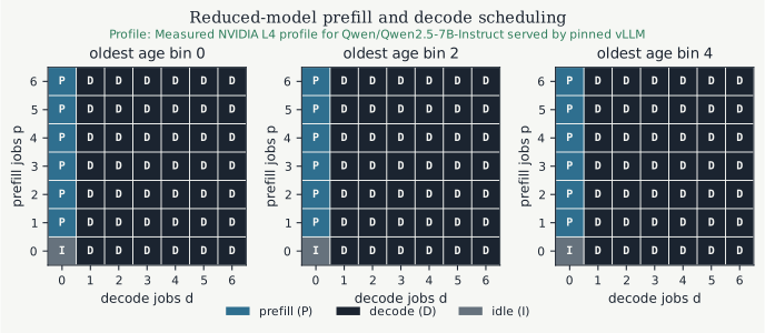
Figure 3:Policy slices at oldest-age bins zero, two, and four. The interactive version adds an age selector and controls for playing, stepping through, and scrubbing a fixed episode sampled from the reduced transition model. The queue trajectory is simulated rather than observed directly from vLLM.
The reduced scheduling MDP has the following transition parameters and value-iteration certificate. The Bellman residual applies only to this finite model.
Download the dynamic-programming certificate (CSV)
Value iteration required 2,454 sweeps on this high-discount problem. Its independently recomputed Bellman residual is , below both the 10-8 acceptance threshold and the 10-10 stopping tolerance. The certificate concerns the supplied 245-state transition matrix. The optimal policy serves decode whenever , serves prefill when and , and idles only in the empty state. The same rule appears in all five age slices. For this calibration, the decode-stall penalty and aggregate completion budget make the transparent decode-priority heuristic exactly optimal within the reduced model. A richer state or a different cost can produce a switching boundary instead.
The result is exact for the stated finite MDP, not for vLLM. Aggregating request ages and lengths removes distinctions that can affect head-of-line waiting and cache release. The calibrated transition kernel is stationary, the clock is fixed, temperature is absent from the state, and the action set excludes mixed prefill-decode batches. Measurements from one L4 deployment calibrate the phase rates and powers; they do not establish scheduling performance across L4 systems. The request-level replay from the earlier chapters remains a model-audit tool, not part of the optimality proof.
Inspect the scheduling MDP and value iteration
1 2 3 4 5 6 7 8 9 10 11 12 13 14 15 16 17 18 19 20 21 22 23 24 25 26 27 28 29 30 31 32 33 34 35 36 37 38 39 40 41 42def solve_scheduling_mdp( mdp: SchedulingMDP | None = None, *, tolerance: float = 1e-10, maximum_iterations: int = 100_000, ) -> DPSolution: """Solve the reduced discounted scheduling model by value iteration.""" model = make_scheduling_mdp() if mdp is None else mdp model.validate() if tolerance <= 0.0 or maximum_iterations <= 0: raise ValueError("tolerance and maximum_iterations must be positive") value = np.zeros(model.states.shape[0], dtype=float) iterations = 0 for iterations in range(1, maximum_iterations + 1): continuation = np.einsum("sak,k->sa", model.transitions, value) q_values = model.stage_cost + model.gamma * continuation q_values = np.where(model.valid_actions, q_values, np.inf) updated = np.min(q_values, axis=1) if np.max(np.abs(updated - value)) <= tolerance: value = updated break value = updated continuation = np.einsum("sak,k->sa", model.transitions, value) q_values = np.where( model.valid_actions, model.stage_cost + model.gamma * continuation, np.inf, ) bellman_update = np.min(q_values, axis=1) residual = float(np.max(np.abs(bellman_update - value))) policy = np.argmin(q_values, axis=1).astype(int) labels = tuple(SCHEDULING_ACTIONS[int(action)] for action in policy) return DPSolution( value=value, policy=policy, policy_labels=labels, iterations=iterations, bellman_residual=residual, mdp=model, )
Newton-Kantorovich Applied to Bellman Optimality
We now apply the Newton-Kantorovich framework to the Bellman optimality equation. Let
The problem is to find such that , or equivalently . The operator is piecewise affine, hence not globally differentiable, but it is directionally differentiable everywhere in the Hadamard sense and Fréchet differentiable at points where the maximizer is unique.
We consider three complementary perspectives for understanding and computing its derivative.
Perspective 1: Max of Affine Maps
In tabular form, for finite state and action spaces, the Bellman operator can be written as a pointwise maximum of affine maps:
where is the transition matrix associated with action . Each is affine in . The operator therefore computes the upper envelope of a finite set of affine functions at each state.
At any , let the active set at state be
Then the Hadamard directional derivative exists and is given by
If the active set is a singleton, this expression becomes linear in , and is Fréchet differentiable at , with
where is the greedy policy at .
Perspective 2: Envelope Theorem
Consider now a value function approximated as a linear combination of basis functions:
At a node , define the parametric maximization
Define
so that . Since is linear in , we can apply the envelope theorem (Danskin’s theorem): if the optimizer is unique or selected measurably, then
We do not need to differentiate the optimizer itself. The result extends to the subdifferential case when ties occur, where the Jacobian becomes set-valued.
This result is useful when solving the collocation equation . Newton’s method requires the Jacobian , and this expression allows us to compute it without involving any derivatives of the optimal action.
Perspective 3: The Implicit Function Theorem
The third perspective applies the implicit function theorem to understand when the Bellman operator is differentiable despite containing a max operator. The maximization problem defines an implicit relationship between the value function and the optimal action, and the implicit function theorem tells us when this relationship is smooth enough to differentiate through.
The Bellman operator is defined as
The difficulty is that the max operator encodes a discrete selection: which action achieves the maximum. To apply the implicit function theorem, we reformulate this as follows. For each action , define the action-value function:
The optimal action at satisfies the optimality condition:
Now suppose that at a particular , action is a strict local maximizer in the sense that there exists such that
This strict inequality is the regularity condition needed for the implicit function theorem. It ensures that the optimal action is unique at and remains so in a neighborhood of .
To see why, consider any perturbation with small. Since is linear in , we have:
The perturbation term is bounded: . Therefore, for , the strict gap ensures that
Thus remains the unique maximizer throughout the neighborhood .
The implicit function theorem now applies: in this neighborhood, the mapping is constant (and hence smooth), taking the value . This allows us to write
as an explicit formula that holds throughout the neighborhood. Since is an affine (hence smooth) function of , we can differentiate it:
More precisely, for any perturbation :
This is the Fréchet derivative:
where is the greedy policy.
The role of the implicit function theorem: It guarantees that when the maximizer is unique with a strict gap (the regularity condition), the argmax function is locally constant, which removes the non-differentiability of the max operator. Without this regularity condition (specifically, at points where multiple actions tie for optimality), the implicit function theorem does not apply, and the operator is not Fréchet differentiable. The active set perspective (Perspective 1) and the envelope theorem (Perspective 2) provide the tools to handle these non-smooth points.
Connection to Policy Iteration
We return to the Newton-Kantorovich step:
Suppose for the greedy policy . Then
which is exactly policy evaluation for . Recomputing the greedy policy from yields the next iterate.
Thus, policy iteration is Newton-Kantorovich applied to the Bellman optimality equation. At points of nondifferentiability (when ties occur), the operator is still semismooth, and policy iteration corresponds to a semismooth Newton method. The envelope theorem is what justifies the simplification of the Jacobian to , bypassing the need to differentiate through the optimizer. This completes the equivalence.
The Semismooth Newton Perspective
The three perspectives we developed above (the active set view, the envelope theorem, and the implicit function theorem) all point toward a deeper framework for understanding Newton-type methods on non-smooth operators. This framework, known as semismooth Newton methods, was developed precisely to handle operators like the Bellman operator that are piecewise smooth but not globally differentiable. The connection between policy iteration and semismooth Newton methods has been rigorously developed in recent work Gargiani et al. (2022).
The classical Newton-Kantorovich method assumes the operator is Fréchet differentiable everywhere. The derivative exists, is unique, and varies continuously with the base point. But the Bellman operator violates this assumption at any value function where multiple actions tie for optimality at some state. At such points, the implicit function theorem fails, and there is no unique Fréchet derivative.
Semismooth Newton methods address this by replacing the notion of a single Jacobian with a generalized derivative that captures the behavior of the operator near non-smooth points. The most commonly used generalized derivative is the Clarke subdifferential, which we can think of as the convex hull of all possible “candidate Jacobians” that arise from limits approaching the non-smooth point from different directions.
For the Bellman residual , the Clarke subdifferential at a point can be characterized explicitly using our first perspective. Recall that at each state , we defined the active set . When this set contains multiple actions, the operator is not Fréchet differentiable. However, it remains directionally differentiable in all directions, and the Clarke subdifferential consists of all matrices of the form
In words, the generalized Jacobian is the set of all matrices where is any policy that selects an action from the active set at each state. When the maximizer is unique everywhere, this set reduces to a singleton, and we recover the classical Fréchet derivative. When ties occur, the set has multiple elements: precisely the convex combinations mentioned in Perspective 1.
The semismooth Newton method for solving proceeds by selecting an element at each iteration and solving
What this tells us is that any choice from the Clarke subdifferential yields a valid Newton-like update. In the context of the Bellman equation, choosing where is any greedy policy corresponds exactly to the policy evaluation step in policy iteration. The freedom in selecting which action to choose when ties occur translates to the freedom in selecting which element of the subdifferential to use.
Under appropriate regularity conditions (specifically, when the residual function is BD-regular or CD-regular), the semismooth Newton method converges locally at a quadratic rate Gargiani et al. (2022). This means that near the solution, the error decreases quadratically:
This theoretical result explains an empirical observation that has long been noted in practice: policy iteration typically converges in very few iterations, often just a handful, even when the state and action spaces are enormous and the space of possible policies is exponentially large.
The semismooth Newton framework also suggests a spectrum of methods interpolating between value iteration and policy iteration. Value iteration can be interpreted as a Newton-like method where we choose at every iteration, ignoring the dependence of on entirely. This choice guarantees global convergence through the contraction property but sacrifices the quadratic local convergence rate. Policy iteration, at the other extreme, uses the full generalized Jacobian , achieving quadratic convergence but at the cost of solving a linear system at each iteration.
Between these extremes lie methods that use approximate Jacobians. One natural variant is to choose for some scalar . This leads to the update
This is known as -value iteration or successive over-relaxation when . For appropriate choices of , this method retains global convergence while achieving better local rates than standard value iteration, and it requires only pointwise operations rather than solving a linear system. The Newton perspective thus unifies existing algorithms and generates new ones by systematically exploring different approximations to the generalized Jacobian.
The connection to semismooth Newton methods places policy iteration within a broader mathematical framework that extends far beyond dynamic programming. Semismooth Newton methods are used in optimization (for complementarity problems and variational inequalities), in PDE-constrained optimization (for problems with control constraints), and in economics (for equilibrium problems). The Bellman equation, viewed through this lens, is simply one instance of a piecewise smooth equation, and the tools developed for such equations apply directly.
Policy Iteration
While we derived policy iteration-like steps from the Newton-Kantorovich method, it’s worth examining policy iteration as a standalone algorithm, as it has been traditionally presented in the field of dynamic programming.
The policy iteration algorithm for discounted Markov decision problems is as follows:
As opposed to value iteration, this algorithm produces a sequence of both deterministic Markovian decision rules and value functions . We recognize in this algorithm the linearization step of the Newton-Kantorovich procedure, which takes place here in the policy evaluation step 3 where we solve the linear system . In practice, this linear system could be solved either using direct methods (eg. Gaussian elimination), using simple iterative methods such as the successive approximation method for policy evaluation, or more sophisticated methods such as GMRES.
Summary and Outlook
Discounting converts an infinite stream of rewards into a bounded value and makes the Bellman maps contractions in the sup norm. Value iteration applies successive approximation; policy iteration alternates a fixed-policy linear solve with greedy improvement. The inference-scheduling example also shows the price of state reduction: a smaller MDP averages over distinctions that can still affect future completions.
The hard maximum in the Bellman operator selects one action and is nondifferentiable at ties. Can the decision rule remain stochastic while the operator becomes smooth? Smooth and regularized dynamic programming answers by placing a convex regularizer on the action distribution.
Self-checks
Solution to Exercise 1
At most . The discounted Bellman operator is a -contraction in the sup norm.
Solution to Exercise 2
.
Solution to Exercise 3
Policy evaluation solves . Policy improvement computes action values from that and chooses a greedy action in each state.
Solution to Exercise 4
Two states can have the same numbers of waiting and decoding requests and the same oldest prefill-age bin while their active requests have different remaining output lengths. The reduced state discards those lengths, so its transition kernel averages over them.
- Puterman, M. L. (1994). Markov Decision Processes: Discrete Stochastic Dynamic Programming. John Wiley & Sons.
- Gargiani, M., Zanelli, A., Liao-McPherson, D., Summers, T. H., & Lygeros, J. (2022). Dynamic Programming Through the Lens of Semismooth Newton-Type Methods. IEEE Control Systems Letters, 6, 2996–3001. 10.1109/LCSYS.2022.3181213