Stochastic dynamic programming chooses a feedback action by minimizing immediate cost plus expected continuation cost. In continuous time, that recursion becomes a partial differential equation for the value function. Can forward simulations compute the optimal action without solving this equation over a grid of states?
For a class of systems with quadratic control effort and matching physical noise, a logarithmic transformation turns the value equation into a linear one. Its solution is an expectation over trajectories, which can be estimated by sampling. This gives conditions under which the weighted updates introduced in the MPPI chapter compute an optimal current feedback action. A particle moving through two competing passages then shows how physical uncertainty can change the preferred route.
Learning Goals
After working through the derivation and experiments, you should be able to:
Derive the stochastic Hamilton--Jacobi--Bellman equation from the short-time Bellman recursion.
State the noise and control-cost matching condition and use it to obtain a path-integral representation of the value function.
Estimate a current feedback action from weighted noise increments, including the correction for a controlled sampling process.
Distinguish an optimal feedback action from a Gaussian fit to a distribution over open-loop control sequences.
Compare stochastic and mean-dynamics controllers using paired disturbances, numerical reference solutions, and discretization checks.
Prerequisites
This chapter uses the Bellman recursion and state-dependent policies from Finite-Horizon Dynamic Programming and Stochastic Dynamic Programming. Gaussian increments are reviewed from Stochastic Dynamics and Partial Observation. The comparison with MPPI uses the Gaussian mean fit and importance-sampling correction in From Trajectory Weights to MPPI. The continuous-time value equation and its transformation are derived below.
Stochastic Feedback Control
How does the Bellman recursion change when controls and disturbances act continuously in time? A scalar model with Gaussian increments gives the noise scaling needed to take the short-time limit. The resulting value function accounts for future actions responding to future observations.
A model with physical noise
Consider a scalar position whose control sets its average velocity over an interval of length . Suppose the motion also has an independent Gaussian displacement during each interval:
Here is the variance of the physical displacement per unit time. Over intervals, the accumulated noise variance is . Thus subdividing a fixed duration into smaller steps preserves the total variance. The factor gives this property: using instead would make the total noise variance vanish as the steps become smaller.
Brownian motion is the continuous-time process that supplies these independent Gaussian increments. If denotes standard Brownian motion, then . The continuous-time model is written
For a control held constant over one interval, integrating this equation gives the Gaussian transition above exactly. The notation denotes an increment of the random process. It is not an ordinary velocity that can be evaluated and multiplied by a time step.
This physical randomness remains even when the control is fixed. A simulator draws independent increments to represent possible futures from the observed state; those draws do not predict the particular disturbance the system will experience. To use the rollout notation from From Trajectory Weights to MPPI, write the same transition as , where . Its variance is because it is multiplied by to produce the physical displacement. In this model, physical noise determines the perturbation covariance used in the path-integral derivation.
The stochastic control problem
Let follow the control-affine diffusion
The drift describes uncontrolled motion, maps the -dimensional control into state motion, and maps Brownian noise into state fluctuations. For the scalar particle, these objects are , , and . Controls may depend on the current state and time, but not on future noise.
For a fixed terminal time , define
The expectation is conditional on and follows the chosen feedback controller. The infimum ranges over controllers whose current action uses only information available at the current time. The value is the smallest expected remaining cost from that state.
Assume the coefficients are sufficiently regular for the diffusion to exist without explosion, the costs are bounded below with finite expectations, and the value function is once continuously differentiable in time and twice in state. These assumptions permit the following classical differential calculation. The control set is , and the noise and effort must satisfy
The equality is pointwise in time and state. It matches both the directions and magnitudes of control and noise. For the scalar Brownian particle, , , and , so . Independent choices of all three quantities would generally violate the equality. Unactuated state coordinates are allowed, but additional independent noise outside the control directions does not satisfy this model.
The stochastic Hamilton--Jacobi--Bellman equation
The stochastic Bellman recursion compares immediate cost with expected optimal continuation cost. Over a short interval , its continuous-time form is:
For this expansion the control is fixed over the short interval. The state increment has mean and covariance . Its second-order contribution therefore survives division by . Expanding the last expectation gives
Subtracting , dividing by , and taking the limit gives the stochastic Hamilton--Jacobi--Bellman (HJB) equation:
For the particle, the diffusion contribution is . Brownian displacements are of order , so their squared displacements contribute at order , the same order as drift and running cost. Omitting the second derivative would replace this stochastic recursion by a deterministic one.
Only the terms inside braces depend on the current action. Since is positive definite, differentiating this strictly convex quadratic gives its unique minimizer:
Substitution removes the minimization and leaves
The term quadratic in makes this equation nonlinear, even though the control minimization itself was explicit.
Path-Integral Representation
Can the nonlinear value equation be transformed into an expectation that we can estimate with forward simulations? The noise-matching condition allows a logarithmic change of variables to cancel the term quadratic in the value gradient. The resulting linear equation has a probabilistic solution.
The logarithmic transformation
The minimized HJB equation contains both a term quadratic in and a diffusion term involving . A logarithm can connect these terms because its second derivative includes a squared first derivative. Define , or equivalently . The positive function is called the desirability: states with lower optimal cost have larger . Its derivatives are
After substitution into HJB, the quadratic terms combine as
Noise matching sets this expression to zero. Multiplying the remaining equation by produces the linear backward equation
This cancellation is the restriction behind the path-integral solution Kappen, 2005. An arbitrary control penalty or arbitrary additional diffusion leaves a nonlinear equation after the transformation.
A forward expectation
The linear equation has a probabilistic solution. Let be the law of trajectories generated by the uncontrolled process . Along one such trajectory, consider
The stochastic chain rule, or Itô’s formula, expands changes in using the same first and second derivatives as the short-time calculation. The drift of is its exponential factor times , which vanishes. Assuming the remaining stochastic integral is integrable and has mean zero, . Using the terminal condition therefore yields
This is the Feynman--Kac representation. The expectation integrates over whole sample paths of the uncontrolled diffusion, hence the name path integral. It replaces a backward partial differential equation with forward simulations starting at the particular state of interest. The quadratic control cost is absent from because its effect is already incorporated through noise matching and the logarithm.
Quadratic cost and optimal feedback
For the scalar particle with terminal cost , with , and no running state cost, the uncontrolled endpoint is , where . The expectation is an ordinary Gaussian integral:
Both terms in the exponent are quadratic in the endpoint . Completing the square with gives
The constant term leaves the integral, and integrating the remaining Gaussian supplies its normalization factor. Using yields
Taking its logarithm and differentiating gives a value and feedback law that can be checked without Monte Carlo:
Noise increases the optimal expected cost through the logarithmic term. For this quadratic example it does not change the feedback law. This is certainty equivalence. Nonquadratic state costs or barriers are needed to observe decisions that depend on the diffusion strength.
At , , , and , the current action is , the mean found in the deterministic quadratic check in From Trajectory Weights to MPPI. Here the controller also responds to later observations by reevaluating at the new state and time. Agreement of the initial actions does not make the execution rules identical. Exercise Exercise 2 verifies the value equation directly.
Sampling the Optimal Action
How can sampled trajectories estimate the feedback action without numerically differentiating the value function? The first noise increment changes both the next state and the expected future cost weight. Their correlation supplies the derivative needed for the current action.
Estimating the control from noise increments
The value representation still appears to require a state derivative to obtain the control. For the particle, however, a positive first noise increment changes the remaining expected weight by approximately . Multiplying by and averaging keeps this term because ; terms constant in the increment average to zero. Thus the correlation of the first increment with the future weight estimates a state derivative.
To express this calculation for several control directions, take to have full column rank and write , with constant invertible satisfying . Conditional on a short initial increment, the remaining expected weight is times the initial running-cost factor. Its first-order expansion and give
The deterministic terms have zero correlation with the mean-zero noise. Dividing by recovers the optimal control:
Low-cost future paths receive greater weight, and their initial random displacements determine which control direction to apply now. The formula is conditional on the specified current state; estimates for future times require the corresponding state conditioning.
Sampling around a controlled trajectory
Uncontrolled simulations may rarely reach the target. Instead, simulate under an adapted sampling control with the same diffusion, and denote the resulting trajectory law by . Girsanov’s change-of-measure formula gives
Here is Brownian motion under the sampling law. Sufficient conditions include the usual exponential-integrability condition , which ensures that this likelihood ratio defines a probability measure. The ratio is the continuous-time counterpart of the Gaussian density expansion in From Trajectory Weights to MPPI: the accumulated squared mean shift supplies the first integral and the mean-noise cross terms supply the second.
Absorb the ratio into a corrected path cost,
Its stochastic integral has mean zero but must remain inside the exponential weight. The control estimator then becomes
The weighted perturbation corrects the current sampling control. The exact result holds for different admissible sampling controls, although their Monte Carlo variances can differ substantially Thijssen & Kappen, 2015.
Discretization and the MPPI update
For simulation with step , Euler--Maruyama gives
The random state increment is , so its covariance is , as required by the diffusion. The input perturbation itself has covariance . Halving therefore increases its standard deviation by , while reducing the standard deviation of the physical state increment by . The two scalings refer to different quantities. Let denote the terminal state cost plus a quadrature approximation of the running state cost. With , approximating the integrals in yields
For a deterministic nominal sequence, the first term inside the sum is common to every rollout and cancels in normalized weights. The remaining cross term is exactly the discrete likelihood correction . For a state-dependent sampling controller, the quadratic term generally varies across trajectories and must be retained.
The weighted perturbation has the same form as the update in From Trajectory Weights to MPPI. That derivation fits a Gaussian to the Gibbs law with density proportional to , where is a reference density over input sequences. Its result and the stochastic control result describe different objects:
| Calculation | Result before numerical approximation | Approximation used in computation |
|---|---|---|
| Gibbs weighting and Gaussian fitting | Mean of , an exact fit within the fixed-covariance Gaussian family | Finite importance samples estimate that mean; fitting discards other features of |
| Matched stochastic control | Optimal current feedback action from the limiting first-noise expectation | Time discretization and finite samples approximate the conditional expectation |
The distributional mean describes an entire open-loop sequence. The stochastic-control formula gives a current feedback action conditioned on a specified state. Its future feedback actions require the future states as well. For general nonlinear constrained models, neither Gaussian averaging nor finite sampling guarantees global optimality or feasibility.
The expectation in the original control objective remains an ordinary expected cost. Exponential weighting over the uncontrolled diffusion solves that objective because of the HJB transformation and noise matching. Exponentiating costs from arbitrary disturbance scenarios of an unrelated model does not establish the same result. In particular, physical disturbance uncertainty and extra numerical exploration must be specified separately whenever the matched diffusion interpretation does not apply.
Brownian Motion Through Competing Passages
When does uncertainty change the direction of the optimal force? The quadratic example cannot answer this question because its optimal action has certainty equivalence. We now keep the same fully observed particle and quadratic effort, and change the geometry of the state cost.
Imagine a particle starting at . Between times 1 and 2, it should stay in one of two openings: a narrow interval near its starting position, or a wider interval farther to the left. One possible trajectory moves right into the narrow opening, stays there while the passage is active, and then approaches the terminal target at time 3. Another moves left into the wider opening and returns toward the target afterward. With weak fluctuations, the shorter route requires less effort. Stronger fluctuations make remaining inside the narrow opening more difficult.
The horizontal coordinate in the figures is time, and the vertical coordinate is the particle’s scalar position. The openings describe a cost that depends on both time and position; they are not a second dynamical state. This construction follows the double-slit and unequal-passage examples of Kappen (2005). The finite penalties and numerical parameters below are adaptations for a runnable teaching example.
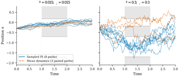
Figure 1:Paired realizations at two physical noise levels. Gray regions incur a finite penalty. Blue paths use sampled path-integral feedback; dashed orange paths use feedback obtained by planning under mean dynamics. The same Brownian increments act on both controllers within each trial. Here and .
A finite-width double slit with an analytic solution
The full passage requires a sequence of successful positions. To isolate the decision about when to choose a route, first replace that duration by a single crossing time . The particle pays a lump penalty if lies outside a union of intervals , and a terminal cost . The diffusion and effort remain
The desirability is the expected exponential weight under uncontrolled Brownian motion, as derived in Stochastic Feedback Control. Conditioning on separates the crossing from the terminal transport:
The quadratic calculation above gives
Multiplying the two Gaussian factors and completing the square leaves a normalized Gaussian in . Write for the time until crossing and for the remaining time after crossing plus the effort-to-terminal-cost ratio. The Gaussian product has mean and variance
The terminal cost pulls its mean toward zero: . Under this cost-weighted Gaussian, the probability of lying in an opening is
where is the standard normal cumulative distribution function. Inside an opening, the crossing weight is one; outside, it is . Averaging these two values gives
This is an analytic benchmark for finite passage widths and a finite penalty. Taking prohibits crossing outside an opening. For symmetric openings shrinking to points at , their equal terminal costs cancel from the control ratio, giving
At , symmetry forces . The response to a small displacement is
If , the force returns a small displacement toward the center: there is time to postpone commitment. If , the force amplifies the displacement toward one opening. A realized fluctuation can then determine which route the feedback follows. At the exact symmetry point, an action of zero expresses symmetry; it does not guarantee that a single realized path will pass through the center of either opening.
![Left: the symmetric narrow-slit limit, with a=\nu=1, changes its response near
x=0 as the crossing approaches. Right: forward importance sampling is checked
against the finite-width formula at x=0.2, using openings [-1.15,-0.85] and
[0.85,1.15], t_s=2, T=3, r=\kappa=\nu=1, and F=20. Each estimate
averages 32 independent batches of 4096 samples; bars show 95% confidence
intervals for that mean.](/rlbook/build/brownian-feedback-5fb028d7e8f563a44c636d26801ac2a0.svg)
Figure 2:Left: the symmetric narrow-slit limit, with , changes its response near as the crossing approaches. Right: forward importance sampling is checked against the finite-width formula at , using openings and , , , , and . Each estimate averages 32 independent batches of 4096 samples; bars show 95% confidence intervals for that mean.
Staying inside unequal passages
A finite-thickness passage requires staying in an opening for a duration. For the geometry in Figure 1, define
We hold fixed and compare with . The matching condition requires changing from 0.015 to 0.3 at the same time. Keeping a separate fixed temperature would change the relationship to this stochastic-control problem.
The simulation uses and evaluates the passage penalty at the right endpoint of each transition. At each decision, the path-integral controller samples 4096 futures up to the end of the passage. The terminal quadratic tail from time 2 to time 3 is integrated analytically. Three Gaussian trajectory proposals generate the futures: one guides the particle toward each opening, and one retains zero drift. Their mixture improves coverage when successful passage trajectories are rare under passive sampling.
The trajectory probability of this mixture must appear in the correction. If is the density of the complete sequence of increments under route , the denominator is . The same route is chosen for an entire simulated future, so a product of per-step mixture densities would describe a different sampling procedure. Let be the joint density of the uncontrolled increments, each distributed as . For sampled increment sequences , normalize the following weights to sum to one and use their weighted first increment to estimate the action:
The guiding routes choose where to sample. The weighted first increment chooses the actual force. The physical Brownian increment applied after this choice comes from a separate random-number stream.
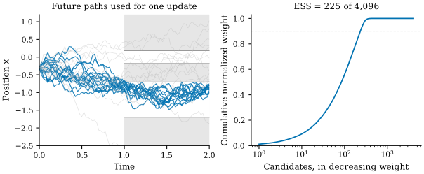
Figure 3:Futures from one high-noise update at . Blue curves are among the highest-weight samples; gray curves have smaller weights. The right panel shows how many samples carry most of the normalized weight. The effective sample size, , diagnoses weight concentration rather than measuring the number of physically possible futures.
An independent reference evaluates the discretized Feynman--Kac expectation by backward Gaussian convolution on a position grid:
Differentiating the Gaussian kernel gives the same first-increment estimator without Monte Carlo sampling. This is a reference for the time-discretized path-integral formula. Executing its force as piecewise constant feedback still introduces a time-step approximation to continuous-time optimal control. We do not identify its finite-step realized cost with the exact continuous-time value.
The comparison controller solves a deterministic dynamic program with the same state cost and control effort, using . This baseline asks what is lost by replacing the future diffusion by its mean. It applies its first action to the observed noisy state and recomputes the action after each step. Both methods therefore use feedback; they differ in whether planning accounts for the future diffusion. The deterministic position grid has spacing 0.0025, corresponding to action spacing 0.1, with a numerical action limit of 24. The reference convolution uses spacing 0.005 on .
Passage choice, cost, and failures
Does accounting for diffusion change which passage is used, and does that choice reduce realized cost? The comparison uses 128 independent physical disturbance sequences, paired across controllers. Pairing gives the methods the same fluctuations, so an apparent improvement cannot be explained by one method receiving an easier collection of disturbances.
| Physical noise | Sampled path-integral cost | Mean-dynamics cost | Numerical-reference cost |
|---|---|---|---|
The entries are means with normal-approximation 95% confidence intervals across trials. The sampled controller and the independent numerical reference give similar mean costs. Mean-dynamics planning has larger cost at both noise levels, even though it also replans from the observed state.
At low noise, neither planning method occupies the wide passage at time 1.5. At high noise, their choices separate:
| Controller, | Wide-passage trials | Wilson 95% interval for the proportion |
|---|---|---|
| Sampled path-integral feedback | ||
| Mean-dynamics planning |
Occupancy includes every trial, including those that incur a penalty. Accounting for the stronger diffusion favors the wider route despite its detour. This is the effect that the quadratic target alone could not show.
A finite penalty still allows failed passages. A trial fails if any checked position lies outside both openings during :
| Physical noise | Sampled path-integral failures | Mean-dynamics failures |
|---|---|---|
At high noise, mean control effort is 1.142 for sampled feedback and 1.531 for mean-dynamics planning. The cost difference includes both the effort and the accumulated penalty for positions outside the passages.
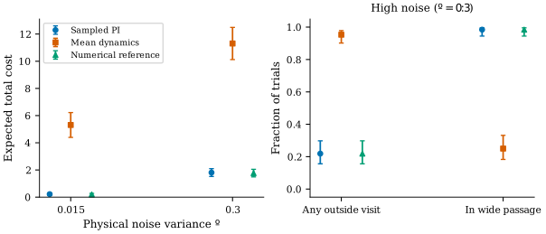
Figure 4:Costs and passage outcomes under paired physical disturbances. Cost bars are 95% intervals for means; proportion bars are Wilson 95% intervals. The numerical reference and the sampled controller have similar outcomes. The finite penalty does not impose a probability-of-failure guarantee.
Sampling error and discretization error
The reference solution lets us vary numerical accuracy separately from physical noise. At the high-noise initial state, increasing the candidate count from 256 to 16384 reduces the first-action root-mean-square error against the convolution reference from 0.910 to 0.103 across 32 independent batches. Refining the time step from 0.05 to 0.00625 changes the reference first action from -0.681 to -0.749. Near the route-switching regime, this sensitivity is larger: for , the same refinement changes the action from -0.173 to -0.412. The finite-grid demonstration should therefore be interpreted at its stated resolution. Crossings between checked times are not counted.
Refining the deterministic grid from 0.0025 to 0.00125 changes its paired mean cost from 5.310 to 4.915 at low noise and from 11.303 to 11.446 at high noise. No executed control reaches the numerical action limit. The cost gap persists under this refinement, although the deterministic baseline itself is not fully converged. Expanding the convolution domain from to leaves its initial high-noise action unchanged to the displayed precision. All settings, trial arrays, and convergence sweeps are retained in the experiment results.
Replay a paired trial, change the physical noise level, and inspect accumulated control effort and outside visits. The replay uses saved trajectories.
The mean-dynamics controller often waits near an opening’s edge. Which term in its predicted objective assigns a cost to remaining close to that edge, and which future events does that prediction omit? The stochastic controller accounts for the cost of correcting future fluctuations, which can favor a wider passage even when reaching it requires more travel.
Summary and Outlook
The stochastic HJB equation is the continuous-time Bellman equation for feedback control under physical noise. With quadratic effort and matching control and noise directions, the logarithmic transformation turns this nonlinear equation into a linear one. The transformed value is an exponential expectation over uncontrolled trajectories, and correlations with the first noise increment give the optimal current action.
Importance sampling allows those trajectories to be drawn around a useful control. Time discretization then produces the weighted-perturbation form used by MPPI. The continuous-time result concerns an action conditioned on the current state; finite samples and a finite time step introduce errors, and a stored sequence still requires replanning to supply feedback.
The quadratic example has certainty equivalence, whereas competing passages make future fluctuations affect the route choice. Paired trials and numerical reference calculations separate that modeling effect from sampling and discretization errors. The matching assumption also limits the theory’s scope: the aircraft optimizer in Aircraft Planning Under Uncertain Winds uses a general distributional fit to estimated expected costs, which by itself does not establish optimal feedback.
Computational Sources
The passage experiments read precomputed results when the book is built. The path sampler and reference calculation have separate implementations:
The Brownian replay displays the recorded simulations without a Python kernel. Regeneration commands are in the repository README.
Exercises
Solution to Exercise 1
(a) Matching requires , hence . The random position increment must have variance . Since it equals , its perturbation variance is .
(b) The variance doubles and the standard deviation increases by . With fixed perturbation variance and duration , the accumulated position variance is , which vanishes as . That discretization approaches deterministic dynamics instead of the prescribed diffusion.
(c) In state order , take and . Then with the value of above. Both noise and control act on velocity, so the unactuated position causes no problem. Independent position noise would add a positive entry to the position variance that the right side cannot represent.
Solution to Exercise 2
(a) Write and , so . Their derivatives are and . Substituting and into cancels both the quadratic and constant terms. At , and , giving the terminal cost.
(b) The feedback is . Only the state-independent term depends on . It increases expected cost but disappears on taking the state derivative.
(c) The cancellation uses the quadratic value function and control-independent additive noise. A state penalty with an obstacle, two separated target regions, or a nonlinear drift need not preserve that structure. For example, two passages with different widths can require different expected control effort to counter diffusion even when their deterministic path lengths are comparable.
Solution to Exercise 3
(a) The calculation uses the within-trial difference:
import numpy as np

with np.load("artifacts/brownian_mppi/trials.npz") as trials:
    for noise in ("low_noise", "high_noise"):
        d = (trials[f"{noise}_path_integral_cost"]
             - trials[f"{noise}_mean_dynamics_cost"])
        half_width = 1.96 * d.std(ddof=1) / np.sqrt(d.size)
        print(noise, d.mean(), half_width)
The mean differences are approximately at low noise and at high noise. Negative values favor path-integral feedback.
(b) This interval describes uncertainty in the estimated mean cost difference across independent trials. An individual realized cost can be far from that mean. Pairing also contributes a covariance term: . Computing the differences preserves the covariance produced by shared physical disturbances; treating the two arrays as independent discards it.
(c) Hold the model, state, time step, and reference grid fixed while varying candidate count across independent sampling seeds. Compare the first action with the backward-convolution action at that time step. Separately, vary the time step in the reference calculation while keeping physical coefficients fixed, including and the corresponding perturbation scaling. These comparisons isolate Monte Carlo error and time resolution. The observed failures and unchecked crossings between time steps rule out a claim of guaranteed passage feasibility.
Self-checks
Solution to Exercise 4
The physical Brownian increments remain. Stopping the sampler removes simulated futures used to estimate an update; it does not change the particle’s process noise.
- Kappen, H. J. (2005). Path integrals and symmetry breaking for optimal control theory. Journal of Statistical Mechanics: Theory and Experiment, 2005(11), P11011. 10.1088/1742-5468/2005/11/P11011
- Thijssen, S., & Kappen, H. J. (2015). Path integral control and state-dependent feedback. Physical Review E, 91(3), 032104. 10.1103/PhysRevE.91.032104