Parametric and Approximate Controllers

Real-time model predictive control places strict limits on computation. In applications such as adaptive optics, the controller must run at kilohertz rates. A sampling frequency of 1000 Hz allows only one millisecond per step to compute and apply a control input. This makes efficiency a first-class concern.

The structure of MPC lends itself naturally to optimization reuse. Each time step requires solving a problem with the same dynamics and constraints. Only the initial state, forecasts, or reference signals change. Instead of treating each instance as a new problem, we can frame MPC as a parametric optimization problem and focus on how the solution evolves with the parameter.

Can the previous solution, its local sensitivity, or a learned approximation replace part of the next online optimization without hiding when that approximation ceases to be valid?

General Framework: Parametric Optimization¶

How do the optimizer and optimal value change as the initial state, forecast, or reference parameter moves?

We begin with a general optimization problem indexed by a parameter $\boldsymbol{\theta} \in \Theta \subset \mathbb{R}^p$:

For each value of $\boldsymbol{\theta}$, we obtain a concrete optimization problem. The goal is to understand how the optimizer $\mathbf{x}^\star(\boldsymbol{\theta})$ and value function

depend on $\boldsymbol{\theta}$.

When the problem is smooth and regular, the Karush–Kuhn–Tucker (KKT) conditions characterize optimality:

If the active set remains fixed over changes in $\boldsymbol{\theta}$, the implicit function theorem ensures that the mappings

are differentiable.

In linear and quadratic programming, this structure becomes even more tractable. Consider a linear program with affine dependence on $\boldsymbol{\theta}$:

Each active set determines a basis and thus a region in $\Theta$ where the solution is affine in $\boldsymbol{\theta}$. The feasible parameter space is partitioned into polyhedral regions, each with its own affine law.

Similarly, in strictly convex quadratic programs

each active set again leads to an affine optimizer, with piecewise-affine global structure and a piecewise-quadratic value function.

Parametric programming focuses on the structure of the map $\boldsymbol{\theta} \mapsto \mathbf{x}^\star(\boldsymbol{\theta})$, and the regions over which this map takes a simple form.

Solution Sensitivity via the Implicit Function Theorem¶

We often meet equations of the form

where $y\in\mathbb{R}^m$ are unknowns and $\boldsymbol{\theta}\in\mathbb{R}^p$ are parameters. The implicit function theorem says that, if $F$ is smooth and the Jacobian with respect to $y$,

is invertible at a solution $(y^\star,\boldsymbol{\theta}^\star)$, then in a neighborhood of $\boldsymbol{\theta}^\star$ there exists a unique smooth mapping $y(\boldsymbol{\theta})$ with $F(y(\boldsymbol{\theta}),\boldsymbol{\theta})=0$ and $y(\boldsymbol{\theta}^\star)=y^\star$. Moreover, its derivative is

In words: if the square Jacobian in $y$ is nonsingular, the solution varies smoothly with the parameter, and we can differentiate it by solving one linear system.

Return to $(P_{\theta})$ and its KKT system. Collect the primal and dual variables into

and write the KKT equations as a single residual

Here $\mathcal{A}$ denotes the set of inequality constraints active at the solution (the complementarity part is encoded by keeping $\mathcal{A}$ fixed; see below).

To invoke IFT, we need the Jacobian $\partial F/\partial y$ to be invertible at $(y^\star,\boldsymbol{\theta}^\star)$. Standard regularity conditions that ensure this are:

• LICQ (Linear Independence Constraint Qualification) at $(\mathbf{x}^\star,\boldsymbol{\theta}^\star)$: the gradients of all active constraints are linearly independent.

• Second-order sufficiency on the critical cone (the Lagrangian Hessian is positive definite on feasible directions).

• Strict complementarity (optional but convenient): each active inequality has strictly positive multiplier.

Under these, the KKT matrix,

is nonsingular. Here $\mathcal{L}=f+\boldsymbol{\lambda}^\top \mathbf{g}+\boldsymbol{\nu}^\top \mathbf{h}$.

The right-hand side sensitivity to parameters is

IFT then gives local differentiability of the optimizer and multipliers:

The formula above is valid as long as the active set $\mathcal{A}$ does not change. If a constraint switches between active/inactive, the mapping remains piecewise smooth, but the derivative may jump. In MPC, this is exactly why warm-starts are very effective most of the time and occasionally require a refactorization when the active set flips.

In parametric MPC, $\boldsymbol{\theta}$ gathers the current state, references, and forecasts. The IFT tells us that, under regularity and a stable active set, the optimal trajectory and first input vary smoothly with $\boldsymbol{\theta}$. The linear map $-K^{-1}G$ is exactly the object used in sensitivity-based warm starts and real-time iterations: small changes in $\boldsymbol{\theta}$ can be propagated through a single KKT solve to update the primal–dual guess before taking one or two Newton/SQP steps.

Predictor-Corrector MPC¶

We start with a smooth root-finding problem

Newton’s method iterates

or equivalently solves the linearized system

Convergence is local and fast when the Jacobian is nonsingular and the initial guess is close.

Now suppose the root depends on a parameter:

We want the solution path $\theta\mapsto y^\star(\theta)$. Numerical continuation advances $\theta$ in small steps and uses the previous solution as a warm start for the next Newton solve. This is the simplest and most effective way to “track” solutions of parametric systems.

At a known solution $(y^\star,\theta^\star)$, differentiate $F(y^\star(\theta),\theta)=0$ with respect to $\theta$:

If $\nabla_y F$ is invertible (IFT conditions), the tangent is

This is exactly the implicit differentiation formula. Continuation uses it as a predictor:

Then a few corrector steps apply Newton to $F(\,\cdot\,,\theta^\star+\Delta\theta)=0$ starting from $y_{\text{pred}}$. If Newton converges quickly, the step $\Delta\theta$ was appropriate; otherwise reduce $\Delta\theta$ and retry.

For parametric KKT systems, set $y=(\mathbf{x},\boldsymbol{\lambda},\boldsymbol{\nu})$ where $\mathbf{x}$ stacks the primal decision variables (states and inputs), and $F(y,\theta)=0$ the KKT residual with $\theta$ collecting state, references, forecasts. The KKT matrix $K=\partial F/\partial y$ and parameter sensitivity $G=\partial F/\partial \theta$ give the tangent

Continuation then becomes:

1. Predictor: $y_{\text{pred}} = y^\star + (\Delta\theta)\,(-K^{-1}G)$.

2. Corrector: a few Newton/SQP steps on the KKT equations at the new $\theta$.

In MPC, this yields efficient warm starts across time. As the parameter $\theta_t$ (current state and references) changes slightly, we predict the new primal-dual point and correct with 1–2 iterations, which is often enough to reach tolerance in real time.

Amortized Optimization and Neural Approximation of Controllers¶

Can a trained function approximate the parametric optimizer closely enough to replace most online solves?

The idea of reusing structure across similar optimization problems is not exclusive to parametric programming. In machine learning, a related concept known as amortized optimization aims to reduce the cost of repeated inference by replacing explicit optimization with a function that has been learned to approximate the solution map. This approach shifts the computational burden from online solving to offline training.

The goal is to construct a function $\hat{\pi}_{\phi}(\boldsymbol{\theta})$, typically parameterized by a neural network, that maps the input $\boldsymbol{\theta}$ to an approximate solution $\hat{z}^\star(\boldsymbol{\theta})$ or control action $\hat{\mathbf{u}}_0^\star(\boldsymbol{\theta})$. Once trained, this map can be evaluated quickly at runtime, with no need to solve an optimization problem explicitly.

Amortized optimization has emerged in several contexts:

• In probabilistic inference, where variational autoencoders (VAEs) amortize the computation of posterior distributions across a dataset.

• In meta-learning, where the objective is to learn a model that generalizes across tasks by internalizing how to adapt.

• In hyperparameter optimization, where learning a surrogate model can guide the search over configuration space efficiently.

This perspective has also begun to influence control. Recent work investigates how to amortize nonlinear MPC (NMPC) policies into neural networks. The training data come from solving many instances of the underlying optimal control problem offline. The resulting neural policy $\hat{\pi}_\phi$ acts as a differentiable, low-latency controller that can generalize to new situations within the training distribution.

Compared to explicit MPC, which partitions the parameter space and stores exact solutions region by region, amortized control smooths over the domain by learning an approximate policy globally. It is less precise, but scalable to high-dimensional problems where enumeration of regions is impossible.

Neural network amortization is advantageous due to the expressivity of these models. However, the challenge is ensuring constraint satisfaction and safety, which are hard to guarantee with unconstrained neural approximators. Hybrid approaches attempt to address this by combining a neural warm-start policy with a final projection step, or by embedding the network within a constrained optimization layer. Other strategies include learning structured architectures that respect known physics or control symmetries.

Imitation Learning Framework¶

Which state distribution and supervised target make an approximate controller match the optimizer where it will actually be deployed? Consider a fixed horizon $N$ and parameter vector $\boldsymbol{\theta}$ encoding the current state, references, and forecasts. The oracle MPC controller solves

The applied action is $\pi^\star(\boldsymbol{\theta}) := \mathbf{u}_0^\star(\boldsymbol{\theta})$. Our goal is to learn a fast surrogate mapping $\hat{\pi}_\phi:\boldsymbol{\theta}\mapsto \hat{\mathbf{u}}_0 \approx \pi^\star(\boldsymbol{\theta})$ that can be evaluated in microseconds, optionally followed by a safety projection layer.

Supervised learning from oracle solutions. One first samples parameters $\boldsymbol{\theta}^{(i)}$ from the operational domain and solves the corresponding NMPC problems offline. The resulting dataset

is then used to train a neural network $\hat{\pi}_\phi$ by minimizing

Once trained, the network acts as a surrogate for the optimizer, providing instantaneous evaluations that approximate the MPC law.

Example: Propofol Infusion Control¶

How does a parametric receding-horizon controller translate a measured patient state into a constrained infusion decision?

This problem explores the control of propofol infusion in total intravenous anesthesia (TIVA). Our presentation follows the problem formulation developped by Sawaguchi et al. (2008). The primary objective is to maintain the desired level of unconsciousness while minimizing adverse reactions and ensuring quick recovery after surgery.

The level of unconsciousness is measured by the Bispectral Index (BIS), which is obtained using an electroencephalography (EEG) device. The BIS ranges from 0 (complete suppression of brain activity) to 100 (fully awake), with the target range for general anesthesia typically between 40 and 60.

The goal is to design a control system that regulates the infusion rate of propofol to maintain the BIS within the target range. This can be formulated as an optimal control problem:

Where:

• $u(t)$ is the propofol infusion rate (mg/kg/h)

• $x_1$, $x_2$, and $x_3$ are the drug concentrations in different body compartments

• $x_e$ is the effect-site concentration

• $k_{ij}$ are rate constants for drug transfer between compartments

• $BIS(t)$ is the Bispectral Index

• $\lambda$ is a regularization parameter penalizing excessive drug use

• $E_0$, $E_{\text{max}}$, $EC_{50}$, and $\gamma$ are parameters of the pharmacodynamic model

The specific dynamics model used in this problem is so-called “Pharmacokinetic-Pharmacodynamic Model” and consists of three main components:

1. Pharmacokinetic Model, which describes how the drug distributes through the body over time. It’s based on a three-compartment model:

   • Central compartment (blood and well-perfused organs)

   • Shallow peripheral compartment (muscle and other tissues)

   • Deep peripheral compartment (fat)

2. Effect Site Model, which represents the delay between drug concentration in the blood and its effect on the brain.

3. Pharmacodynamic Model that relates the effect-site concentration to the observed BIS.

The propofol infusion control problem presents several interesting challenges from a research perspective. First, there is a delay in how fast the drug can reach a different compartments in addition to the BIS measurements which can lag. This could lead to instability if not properly addressed in the control design.

Furthermore, every patient is different from another. Hence, we cannot simply learn a single controller offline and hope that it will generalize to an entire patient population. We will account for this variability through Model Predictive Control (MPC) and dynamically adapt to the model mismatch through replanning. How a patient will react to a given dose of drug also varies and must be carefully controlled to avoid overdoses. This adds an additional layer of complexity since we have to incorporate safety constraints. Finally, the patient might suddenly change state, for example due to surgical stimuli, and the controller must be able to adapt quickly to compensate for the disturbance to the system.

Source

#  label: fig-mpc-propofol
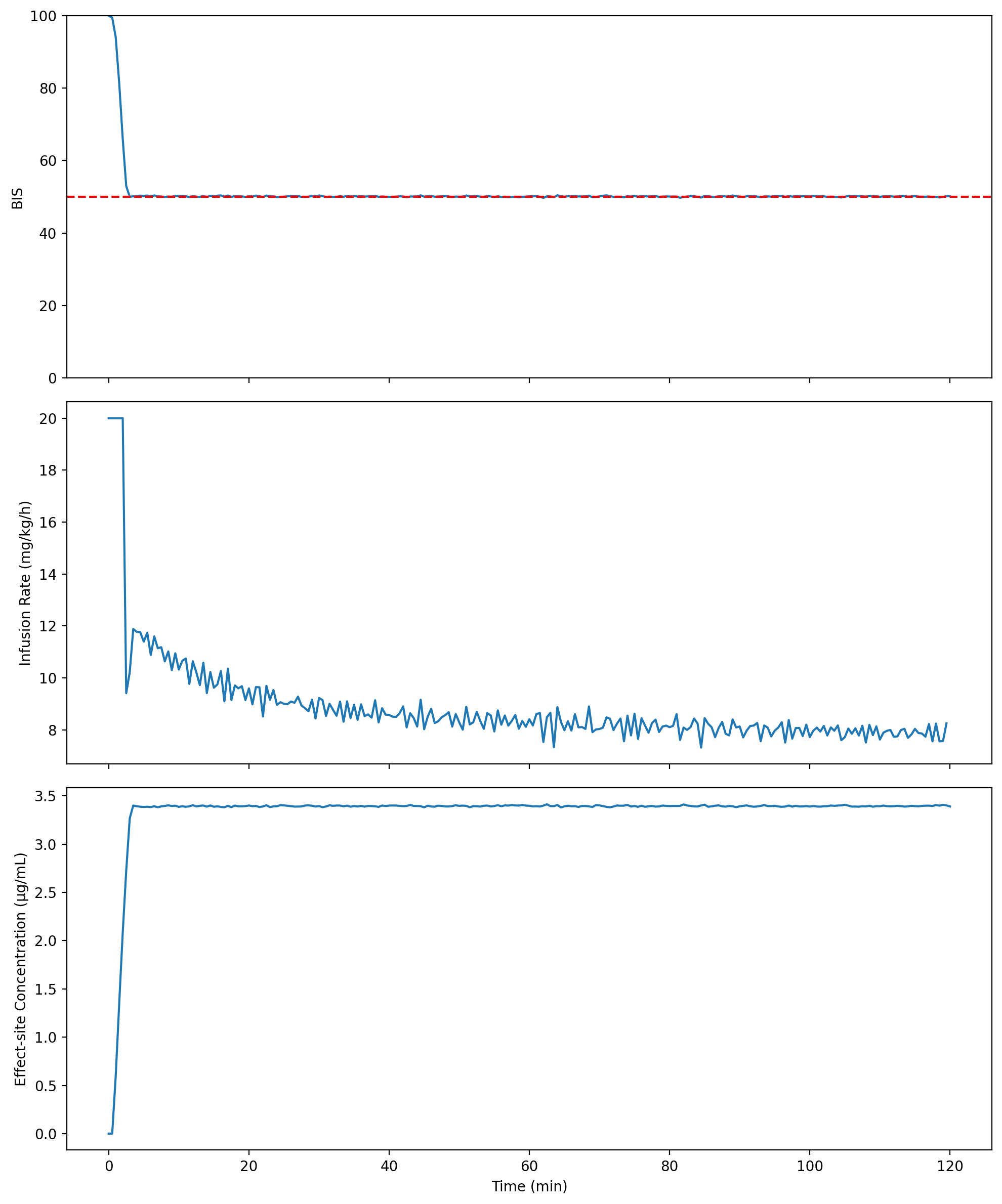
#  caption: Closed-loop MPC for propofol infusion keeps the Bispectral Index near the target (top), regulates infusion rates (middle), and tracks the effect-site concentration (bottom).

%config InlineBackend.figure_format = 'retina'
import numpy as np
from scipy.optimize import minimize
import matplotlib.pyplot as plt

# Apply book style
try:
    import scienceplots
    plt.style.use(['science', 'notebook'])
except (ImportError, OSError):
    pass  # Use matplotlib defaults

class Patient:
    def __init__(self, age, weight):
        self.age = age
        self.weight = weight
        self.set_pk_params()
        self.set_pd_params()

    def set_pk_params(self):
        self.v1 = 4.27 * (self.weight / 70) ** 0.71 * (self.age / 30) ** (-0.39)
        self.v2 = 18.9 * (self.weight / 70) ** 0.64 * (self.age / 30) ** (-0.62)
        self.v3 = 238 * (self.weight / 70) ** 0.95
        self.cl1 = 1.89 * (self.weight / 70) ** 0.75 * (self.age / 30) ** (-0.25)
        self.cl2 = 1.29 * (self.weight / 70) ** 0.62
        self.cl3 = 0.836 * (self.weight / 70) ** 0.77
        self.k10 = self.cl1 / self.v1
        self.k12 = self.cl2 / self.v1
        self.k13 = self.cl3 / self.v1
        self.k21 = self.cl2 / self.v2
        self.k31 = self.cl3 / self.v3
        self.ke0 = 0.456

    def set_pd_params(self):
        self.E0 = 100
        self.Emax = 100
        self.EC50 = 3.4
        self.gamma = 3

def pk_model(x, u, patient):
    x1, x2, x3, xe = x
    dx1 = -(patient.k10 + patient.k12 + patient.k13) * x1 + patient.k21 * x2 + patient.k31 * x3 + u / patient.v1
    dx2 = patient.k12 * x1 - patient.k21 * x2
    dx3 = patient.k13 * x1 - patient.k31 * x3
    dxe = patient.ke0 * (x1 - xe)
    return np.array([dx1, dx2, dx3, dxe])

def pd_model(ce, patient):
    return patient.E0 - patient.Emax * (ce ** patient.gamma) / (ce ** patient.gamma + patient.EC50 ** patient.gamma)

def simulate_step(x, u, patient, dt):
    x_next = x + dt * pk_model(x, u, patient)
    bis = pd_model(x_next[3], patient)
    return x_next, bis

def objective(u, x0, patient, dt, N, target_bis):
    x = x0.copy()
    total_cost = 0
    for i in range(N):
        x, bis = simulate_step(x, u[i], patient, dt)
        total_cost += (bis - target_bis)**2 + 0.1 * u[i]**2
    return total_cost

def mpc_step(x0, patient, dt, N, target_bis):
    u0 = 10 * np.ones(N)  # Initial guess
    bounds = [(0, 20)] * N  # Infusion rate between 0 and 20 mg/kg/h
    
    result = minimize(objective, u0, args=(x0, patient, dt, N, target_bis),
                      method='SLSQP', bounds=bounds)
    
    return result.x[0]  # Return only the first control input

def run_mpc_simulation(patient, T, dt, N, target_bis):
    rng = np.random.default_rng(2026)
    steps = int(T / dt)
    x = np.zeros((steps+1, 4))
    bis = np.zeros(steps+1)
    u = np.zeros(steps)
    
    for i in range(steps):
        # Add noise to the current state to simulate real-world uncertainty
        x_noisy = x[i] + rng.normal(0, 0.01, size=4)
        
        # Use noisy state for MPC planning
        u[i] = mpc_step(x_noisy, patient, dt, N, target_bis)
        
        # Evolve the true state using the deterministic model
        x[i+1], bis[i] = simulate_step(x[i], u[i], patient, dt)
    
    bis[-1] = pd_model(x[-1, 3], patient)
    return x, bis, u

# Set up the problem
patient = Patient(age=40, weight=70)
T = 120  # Total time in minutes
dt = 0.5  # Time step in minutes
N = 20  # Prediction horizon
target_bis = 50  # Target BIS value

# Run MPC simulation
x, bis, u = run_mpc_simulation(patient, T, dt, N, target_bis)

# Plot results
t = np.arange(0, T+dt, dt)
fig, (ax1, ax2, ax3) = plt.subplots(3, 1, figsize=(10, 12), sharex=True)

ax1.plot(t, bis)
ax1.set_ylabel('BIS')
ax1.set_ylim(0, 100)
ax1.axhline(y=target_bis, color='r', linestyle='--')

ax2.plot(t[:-1], u)
ax2.set_ylabel('Infusion Rate (mg/kg/h)')

ax3.plot(t, x[:, 3])
ax3.set_ylabel('Effect-site Concentration (µg/mL)')
ax3.set_xlabel('Time (min)')

plt.tight_layout()

print(f"Initial BIS: {bis[0]:.2f}")
print(f"Final BIS: {bis[-1]:.2f}")
print(f"Mean infusion rate: {np.mean(u):.2f} mg/kg/h")
print(f"Final effect-site concentration: {x[-1, 3]:.2f} µg/mL")

Initial BIS: 100.00
Final BIS: 50.20
Mean infusion rate: 8.86 mg/kg/h
Final effect-site concentration: 3.39 µg/mL

Summary and Outlook¶

Parametric optimization treats successive MPC problems as members of one family rather than unrelated nonlinear programs. Sensitivity updates, predictor-corrector steps, and learned controller approximations trade online optimization time against approximation error and the need to detect a change of active set or operating regime.

MPC has now produced closed-loop behavior by solving a new finite-horizon problem after each observation. Can state-contingent decisions instead be computed across a family of possible states before the next state is known? Finite-horizon dynamic programming begins that second construction of feedback.