Stochastic Dynamic Programming and Markov Decision Processes

Finite-horizon dynamic programming chooses an action from each state and time, then follows one deterministic successor. How should the recursion change when an action induces a distribution of successors and the decision rule itself may be randomized or depend on history? Stochastic dynamic programming answers by averaging continuation values under a transition kernel.

Decision Rules and Policies¶

Which combinations of state, history, and randomization may a decision rule use when selecting an action?

Before diving into stochastic systems, we need to establish terminology for the different types of strategies a decision maker might employ. In the deterministic setting, we implicitly used feedback controllers of the form $u(\mathbf{x}, t)$. In the stochastic setting, we must be more precise about what information policies can use and how they select actions.

A decision rule is a prescription for action selection in each state at a specified decision epoch. These rules can vary in their complexity based on two main criteria:

1. Dependence on history: Markovian or History-dependent

2. Action selection method: Deterministic or Randomized

Markovian decision rules depend only on the current state, while history-dependent rules consider the entire sequence of past states and actions. Formally, a history $h_t$ at time $t$ is:

The set of all possible histories at time $t$, denoted $H_t$, grows exponentially with $t$:

• $H_1 = \mathcal{S}$ (just the initial state)

• $H_2 = \mathcal{S} \times \mathcal{A} \times \mathcal{S}$

• $H_t = \mathcal{S} \times (\mathcal{A} \times \mathcal{S})^{t-1}$

Deterministic rules select an action with certainty, while randomized rules specify a probability distribution over the action space.

These classifications lead to four types of decision rules:

1. Markovian Deterministic (MD): $\pi_t: \mathcal{S} \rightarrow \mathcal{A}_s$

2. Markovian Randomized (MR): $\pi_t: \mathcal{S} \rightarrow \mathcal{P}(\mathcal{A}_s)$

3. History-dependent Deterministic (HD): $\pi_t: H_t \rightarrow \mathcal{A}_s$

4. History-dependent Randomized (HR): $\pi_t: H_t \rightarrow \mathcal{P}(\mathcal{A}_s)$

where $\mathcal{P}(\mathcal{A}_s)$ denotes the set of probability distributions over $\mathcal{A}_s$.

A policy $\boldsymbol{\pi}$ is a sequence of decision rules, one for each decision epoch:

The set of all policies of class $K$ (where $K \in \{HR, HD, MR, MD\}$) is denoted as $\Pi^K$. These policy classes form a hierarchy:

The largest set $\Pi^{HR}$ contains all possible policies. We ask: under what conditions can we restrict attention to the much simpler set $\Pi^{MD}$ without loss of optimality?

Stochastic System Dynamics¶

How does a transition kernel replace the single deterministic successor in the finite-horizon model?

In the stochastic setting, our system evolution takes the form:

Here, $\mathbf{w}_t$ represents a random disturbance or noise term at time $t$ due to the inherent uncertainty in the system’s behavior. The stage cost function may also incorporate stochastic influences:

In this context, our objective shifts from minimizing a deterministic cost to minimizing the expected total cost:

where the expectation is taken over the distributions of the random variables $\mathbf{w}_t$. The principle of optimality still holds in the stochastic case, but Bellman’s optimality equation now involves an expectation:

In practice, this expectation is often computed by discretizing the distribution of $\mathbf{w}_k$ when the set of possible disturbances is very large or even continuous. Let’s say we approximate the distribution with $K$ discrete values $\mathbf{w}_k^i$, each occurring with probability $p_k^i$. Then our Bellman equation becomes:

Optimality Equations in the Stochastic Setting¶

How is the deterministic continuation value replaced by an expectation over all possible next states?

When dealing with stochastic systems, a central question arises: what information should our control policy use? In the most general case, a policy might use the entire history of observations and actions. However, as we’ll see, the Markovian structure of our problems allows for dramatic simplifications.

Let $h_t = (s_1, a_1, s_2, a_2, \ldots, s_{t-1}, a_{t-1}, s_t)$ denote the complete history up to time $t$. In the stochastic setting, the history-based optimality equations become:

where we now explicitly use the transition probabilities $p_t(j|s_t,a)$ rather than a deterministic dynamics function.

Intuition: This formalizes Bellman’s principle of optimality: “An optimal policy has the property that whatever the initial state and initial decision are, the remaining decisions must constitute an optimal policy with regard to the state resulting from the first decision.” The recursive structure means that optimal local decisions (choosing the best action at each step) lead to global optimality, even with uncertainty captured by the transition probabilities.

A simplification occurs when we examine these history-based equations more closely. The Markov property of our system dynamics and rewards means that the optimal return actually depends on the history only through the current state:

Intuition: The Markov property means that the current state contains all information needed to predict future evolution. The past provides no additional value for decision-making. This result allows us to work with value functions $v_t^*(s)$ indexed only by state and time, dramatically simplifying both theory and computation.

This state-sufficiency result, combined with the fact that randomization never helps when maximizing expected returns, leads to a dramatic simplification of the policy space:

Intuition: Even in stochastic systems, randomization in the policy doesn’t help when maximizing expected returns: you should always choose the action with the highest expected value. Combined with state sufficiency, this means simple state-to-action mappings are optimal.

These results justify focusing on deterministic Markov policies and lead to the backward recursion algorithm for stochastic systems:

While SDP provides us with a framework to for handling uncertainty, it makes the curse of dimensionality even more difficult to handle in practice. Both the state space and the disturbance space must be discretized. This can lead to a combinatorial explosion in the number of scenarios to be evaluated at each stage.

However, just as we tackled the challenges of continuous state spaces with discretization and interpolation, we can devise efficient methods to handle the additional complexity of evaluating expectations. This problem essentially becomes one of numerical integration. When the set of disturbances is continuous (as is often the case with continuous state spaces), we enter a domain where numerical quadrature methods could be applied. But these methods tend to scale poorly as the number of dimensions grows. This is where more efficient techniques, often rooted in Monte Carlo methods, come into play. Two ingredients tackle the curse of dimensionality:

1. Function approximation (through discretization, interpolation, neural networks, etc.)

2. Monte Carlo integration (simulation)

These two elements essentially distill the key ingredients of machine learning, which is the direction we’ll be exploring in this course.

Example: Stochastic Optimal Harvest in Resource Management¶

How does uncertain growth change the harvest policy and the distribution of realized returns?

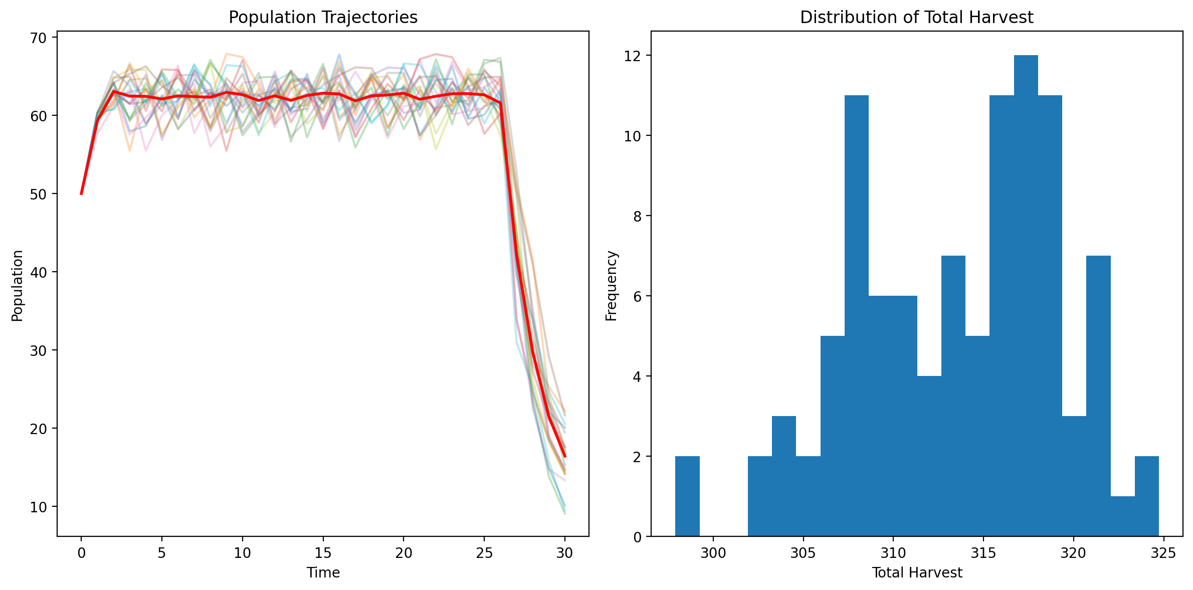
Building upon our previous deterministic model, we now introduce stochasticity to more accurately reflect the uncertainties inherent in real-world resource management scenarios Conroy & Peterson, 2013. As before, we consider a population of a particular species, whose abundance we denote by $x_t$, where $t$ represents discrete time steps. Our objective remains to maximize the cumulative harvest over a finite time horizon, while also considering the long-term sustainability of the population. However, we now account for two sources of stochasticity: partial controllability of harvest and environmental variability affecting growth rates. The optimization problem can be formulated as:

Here, $F(\cdot)$ represents the immediate reward function associated with harvesting, and $h_t$ is the realized harvest rate at time $t$. The expectation $\mathbb{E}[\cdot]$ over both harvest and growth rates, which we view as random variables. In our stochastic model, the abundance $x$ still ranges from 1 to 100 individuals. The decision variable is now the desired harvest rate $d_t$, which can take values from the set $D = {0, 0.1, 0.2, 0.3, 0.4, 0.5}$. However, the realized harvest rate $h_t$ is stochastic and follows a discrete distribution:

By expressing the harvest rate as a random variable, we mean to capture the fact that harvesting is a not completely under our control: we might obtain more or less what we had intended to. Furthermore, we generalize the population dynamics to the stochastic case via:

$$

x_{t+1} = x_t + r_tx_t(1 - x_t/K) - h_tx_t $$

where $K = 125$ is the carrying capacity. The growth rate $r_t$ is now stochastic and follows a discrete distribution:

where $r_{\text{max}} = 0.3$ is the maximum growth rate. Applying the principle of optimality, we can express the optimal value function $J^\star(x_t, t)$ recursively:

where the expectation is taken over the harvest and growth rate random variables. The boundary condition remains $J^*(x_{t_f}) = 0$. We can now adapt our previous code to account for the stochasticity in our model. One important difference is that simulating a solution in this context requires multiple realizations of our process. This is an important consideration when evaluating reinforcement learning methods in practice, as success cannot be claimed based on a single successful trajectory.

Source

#  label: dp-harvest-stochastic
#  caption: Stochastic resource management simulation: the cell reports the optimal policy sample, average trajectory, and visualizes ensemble trajectories plus the distribution of total harvest.

import numpy as np
from scipy.interpolate import interp1d

rng = np.random.default_rng(2026)

# Parameters
r_max = 0.3
K = 125
T = 30  # Number of time steps
N_max = 100  # Maximum population size to consider
h_max = 0.5  # Maximum harvest rate
h_step = 0.1  # Step size for harvest rate

# Create state and decision spaces
N_space = np.linspace(1, N_max, 100)  # Using more granular state space
h_space = np.arange(0, h_max + h_step, h_step)

# Stochastic parameters
h_outcomes = np.array([0.75, 1.0, 1.25])
h_probs = np.array([0.25, 0.5, 0.25])
r_outcomes = np.array([0.85, 1.05, 1.15]) * r_max
r_probs = np.array([0.25, 0.5, 0.25])

# Initialize value function and policy
V = np.zeros((T + 1, len(N_space)))
policy = np.zeros((T, len(N_space)))

# State return function (F)
def state_return(N, h):
    return N * h

# State dynamics function (stochastic)
def state_dynamics(N, h, r):
    return N + r * N * (1 - N / K) - h * N

# Function to create interpolation function for a given time step
def create_interpolator(V_t, N_space):
    return interp1d(N_space, V_t, kind='linear', bounds_error=False, fill_value=(V_t[0], V_t[-1]))

# Backward iteration with stochastic dynamics
for t in range(T - 1, -1, -1):
    interpolator = create_interpolator(V[t+1], N_space)
    
    for i, N in enumerate(N_space):
        max_value = float('-inf')
        best_h = 0

        for h in h_space:
            if h > 1:  # Ensure harvest rate doesn't exceed 100%
                continue

            expected_value = 0
            for h_factor, h_prob in zip(h_outcomes, h_probs):
                for r_factor, r_prob in zip(r_outcomes, r_probs):
                    realized_h = h * h_factor
                    realized_r = r_factor

                    next_N = state_dynamics(N, realized_h, realized_r)
                    if next_N < 1:  # Ensure population doesn't go extinct
                        continue

                    # Use interpolation to get the value for next_N
                    value = state_return(N, realized_h) + interpolator(next_N)
                    expected_value += value * h_prob * r_prob

            if expected_value > max_value:
                max_value = expected_value
                best_h = h

        V[t, i] = max_value
        policy[t, i] = best_h

# Function to simulate the optimal policy using interpolation (stochastic version)
def simulate_optimal_policy(initial_N, T, num_simulations=100):
    all_trajectories = []
    all_harvests = []

    for _ in range(num_simulations):
        trajectory = [initial_N]
        harvests = []

        for t in range(T):
            N = trajectory[-1]
            
            # Create interpolator for the policy at time t
            policy_interpolator = interp1d(N_space, policy[t], kind='linear', bounds_error=False, fill_value=(policy[t][0], policy[t][-1]))
            
            intended_h = policy_interpolator(N)
            
            # Apply stochasticity
            h_factor = rng.choice(h_outcomes, p=h_probs)
            r_factor = rng.choice(r_outcomes, p=r_probs)
            
            realized_h = intended_h * h_factor
            harvests.append(N * realized_h)

            next_N = state_dynamics(N, realized_h, r_factor)
            trajectory.append(next_N)

        all_trajectories.append(trajectory)
        all_harvests.append(harvests)

    return all_trajectories, all_harvests

# Example usage
initial_N = 50
trajectories, harvests = simulate_optimal_policy(initial_N, T)

# Calculate average trajectory and total harvest
avg_trajectory = np.mean(trajectories, axis=0)
avg_total_harvest = np.mean([sum(h) for h in harvests])

print("Optimal policy (first few rows):")
print(policy[:5])
print("\nAverage population trajectory:", avg_trajectory)
print("Average total harvest:", avg_total_harvest)

# Plot results
%config InlineBackend.figure_format = 'retina'
import matplotlib.pyplot as plt

# Apply book style
try:
    import scienceplots
    plt.style.use(['science', 'notebook'])
except (ImportError, OSError):
    pass  # Use matplotlib defaults

plt.figure(figsize=(12, 6))
plt.subplot(121)
for traj in trajectories[:20]:  # Plot first 20 trajectories
    plt.plot(range(T+1), traj, alpha=0.3)
plt.plot(range(T+1), avg_trajectory, 'r-', linewidth=2)
plt.title('Population Trajectories')
plt.xlabel('Time')
plt.ylabel('Population')

plt.subplot(122)
plt.hist([sum(h) for h in harvests], bins=20)
plt.title('Distribution of Total Harvest')
plt.xlabel('Total Harvest')
plt.ylabel('Frequency')

plt.tight_layout()

Optimal policy (first few rows):
[[0.  0.  0.  0.  0.  0.  0.  0.  0.  0.  0.  0.  0.  0.  0.  0.  0.  0.
  0.  0.  0.  0.  0.  0.  0.  0.  0.  0.  0.  0.  0.  0.  0.  0.  0.  0.
  0.  0.  0.  0.  0.  0.  0.  0.  0.  0.  0.  0.  0.  0.  0.  0.  0.  0.
  0.  0.1 0.1 0.1 0.1 0.1 0.1 0.1 0.2 0.2 0.2 0.2 0.2 0.2 0.2 0.2 0.2 0.3
  0.3 0.3 0.3 0.3 0.3 0.3 0.3 0.3 0.3 0.3 0.3 0.3 0.4 0.4 0.4 0.4 0.4 0.4
  0.4 0.4 0.4 0.4 0.4 0.4 0.4 0.4 0.4 0.4]
 [0.  0.  0.  0.  0.  0.  0.  0.  0.  0.  0.  0.  0.  0.  0.  0.  0.  0.
  0.  0.  0.  0.  0.  0.  0.  0.  0.  0.  0.  0.  0.  0.  0.  0.  0.  0.
  0.  0.  0.  0.  0.  0.  0.  0.  0.  0.  0.  0.  0.  0.  0.  0.  0.  0.
  0.  0.1 0.1 0.1 0.1 0.1 0.1 0.1 0.2 0.2 0.2 0.2 0.2 0.2 0.2 0.2 0.2 0.3
  0.3 0.3 0.3 0.3 0.3 0.3 0.3 0.3 0.3 0.3 0.3 0.3 0.4 0.4 0.4 0.4 0.4 0.4
  0.4 0.4 0.4 0.4 0.4 0.4 0.4 0.4 0.4 0.4]
 [0.  0.  0.  0.  0.  0.  0.  0.  0.  0.  0.  0.  0.  0.  0.  0.  0.  0.
  0.  0.  0.  0.  0.  0.  0.  0.  0.  0.  0.  0.  0.  0.  0.  0.  0.  0.
  0.  0.  0.  0.  0.  0.  0.  0.  0.  0.  0.  0.  0.  0.  0.  0.  0.  0.
  0.  0.1 0.1 0.1 0.1 0.1 0.1 0.1 0.2 0.2 0.2 0.2 0.2 0.2 0.2 0.2 0.2 0.3
  0.3 0.3 0.3 0.3 0.3 0.3 0.3 0.3 0.3 0.3 0.3 0.3 0.4 0.4 0.4 0.4 0.4 0.4
  0.4 0.4 0.4 0.4 0.4 0.4 0.4 0.4 0.4 0.4]
 [0.  0.  0.  0.  0.  0.  0.  0.  0.  0.  0.  0.  0.  0.  0.  0.  0.  0.
  0.  0.  0.  0.  0.  0.  0.  0.  0.  0.  0.  0.  0.  0.  0.  0.  0.  0.
  0.  0.  0.  0.  0.  0.  0.  0.  0.  0.  0.  0.  0.  0.  0.  0.  0.  0.
  0.  0.1 0.1 0.1 0.1 0.1 0.1 0.1 0.2 0.2 0.2 0.2 0.2 0.2 0.2 0.2 0.2 0.3
  0.3 0.3 0.3 0.3 0.3 0.3 0.3 0.3 0.3 0.3 0.3 0.3 0.4 0.4 0.4 0.4 0.4 0.4
  0.4 0.4 0.4 0.4 0.4 0.4 0.4 0.4 0.4 0.4]
 [0.  0.  0.  0.  0.  0.  0.  0.  0.  0.  0.  0.  0.  0.  0.  0.  0.  0.
  0.  0.  0.  0.  0.  0.  0.  0.  0.  0.  0.  0.  0.  0.  0.  0.  0.  0.
  0.  0.  0.  0.  0.  0.  0.  0.  0.  0.  0.  0.  0.  0.  0.  0.  0.  0.
  0.  0.1 0.1 0.1 0.1 0.1 0.1 0.1 0.2 0.2 0.2 0.2 0.2 0.2 0.2 0.2 0.2 0.3
  0.3 0.3 0.3 0.3 0.3 0.3 0.3 0.3 0.3 0.3 0.3 0.3 0.4 0.4 0.4 0.4 0.4 0.4
  0.4 0.4 0.4 0.4 0.4 0.4 0.4 0.4 0.4 0.4]]

Average population trajectory: [50.         59.315      63.05075554 62.44820296 62.42420013 62.08230114
 62.48912074 62.38525648 62.30572025 62.92791959 62.63807851 61.8843089
 62.49390308 61.90724971 62.54202248 62.82646214 62.72525486 61.84964529
 62.48319799 62.59056227 62.81887677 62.05344894 62.43721639 62.75546564
 62.76975159 62.61454886 61.56668355 42.12757241 29.72876407 21.52260235
 16.43615057]
Average total harvest: 313.49385676447304

Markov Decision Process Formulation¶

Which state, action, transition, reward, and horizon objects define the common finite MDP representation?

Rather than expressing the stochasticity in our system through a disturbance term as a parameter to a deterministic difference equation, we often work with an alternative representation (more common in operations research) which uses the Markov Decision Process formulation. The idea is that when we model our system in this way with the disturbance term being drawn indepently of the previous stages, the induced trajectory are those of a Markov chain. Hence, we can re-cast our control problem in that language, leading to the so-called Markov Decision Process framework in which we express the system dynamics in terms of transition probabilities rather than explicit state equations. In this framework, we express the probability that the system is in a given state using the transition probability function:

This function gives the probability of transitioning to state $\mathbf{x}_{t+1}$ at time $t+1$, given that the system is in state $\mathbf{x}_t$ and action $\mathbf{u}_t$ is taken at time $t$. Therefore, $p_t$ specifies a conditional probability distribution over the next states: namely, the sum (for discrete state spaces) or integral over the next state should be 1.

Given the control theory formulation of our problem via a deterministic dynamics function and a noise term, we can derive the corresponding transition probability function through the following relationship:

Here, $q_t(\mathbf{w})$ represents the probability density or mass function of the disturbance $\mathbf{W}_t$ (assuming discrete state spaces). When dealing with continuous spaces, the above expression simply contains an integral rather than a summation.

For a system with deterministic dynamics and no disturbance, the transition probabilities become much simpler and be expressed using the indicator function. Given a deterministic system with dynamics:

The transition probability function can be expressed as:

With this transition probability function, we can recast our Bellman optimality equation:

Here, ${c}(\mathbf{x}_t, \mathbf{u}_t)$ represents the expected immediate reward (or negative cost) when in state $\mathbf{x}_t$ and taking action $\mathbf{u}_t$ at time $t$. The summation term computes the expected optimal value for the future states, weighted by their transition probabilities.

This formulation offers several advantages:

1. It makes the Markovian nature of the problem explicit: the future state depends only on the current state and action, not on the history of states and actions.

2. For discrete-state problems, the entire system dynamics can be specified by a set of transition matrices, one for each possible action.

3. It allows us to bridge the gap with the wealth of methods in the field of probabilistic graphical models and statistical machine learning techniques for modelling and analysis.

Notation in Operations Reseach¶

How do equivalent reward, cost, transition, and policy conventions map across reinforcement learning and operations research?

The presentation above was intended to bridge the gap between the control-theoretic perspective and the world of closed-loop control through the idea of determining the value function of a parametric optimal control problem. We then saw how the backward induction procedure was applicable to both the deterministic and stochastic cases by taking the expectation over the disturbance variable. We then said that we can alternatively work with a representation of our system where instead of writing our model as a deterministic dynamics function taking a disturbance as an input, we would rather work directly via its transition probability function, which gives rise to the Markov chain interpretation of our system in simulation.

Note that the notation used in control theory tends to differ from that found in operations research communities, in which the field of dynamic programming flourished. We summarize those (purely notational) differences in this section.

In operations research, the system state at each decision epoch is typically denoted by $s \in \mathcal{S}$, where $S$ is the set of possible system states. When the system is in state $s$, the decision maker may choose an action $a$ from the set of allowable actions $\mathcal{A}_s$. The union of all action sets is denoted as $\mathcal{A} = \bigcup_{s \in \mathcal{S}} \mathcal{A}_s$.

The dynamics of the system are described by a transition probability function $p_t(j | s, a)$, which represents the probability of transitioning to state $j \in \mathcal{S}$ at time $t+1$, given that the system is in state $s$ at time $t$ and action $a \in \mathcal{A}_s$ is chosen. This transition probability function satisfies:

It’s worth noting that in operations research, we typically work with reward maximization rather than cost minimization, which is more common in control theory. However, we can easily switch between these perspectives by simply negating the quantity. That is, maximizing a reward function is equivalent to minimizing its negative, which we would then call a cost function.

The reward function is denoted by $r_t(s, a)$, representing the reward received at time $t$ when the system is in state $s$ and action $a$ is taken. In some cases, the reward may also depend on the next state, in which case it is denoted as $r_t(s, a, j)$. The expected reward can then be computed as:

Combined together, these elemetns specify a Markov decision process, which is fully described by the tuple:

where $\mathrm{T}$ represents the set of decision epochs (the horizon).

What is an Optimal Policy?¶

Against which competing policy class and initial states must a policy be compared before it can be called optimal?

Let’s go back to the starting point and define what it means for a policy to be optimal in a Markov Decision Problem. For this, we will be considering different possible search spaces (policy classes) and compare policies based on the ordering of their value from any possible start state. The value of a policy $\boldsymbol{\pi}$ (optimal or not) is defined as the expected total reward obtained by following that policy from a given starting state. Formally, for a finite-horizon MDP with $N$ decision epochs, we define the value function $v^{\boldsymbol{\pi}}(s, t)$ as:

where $S_t$ is the state at time $t$, $A_t$ is the action taken at time $t$, and $r_t$ is the reward function. For simplicity, we write $v^{\boldsymbol{\pi}}(s)$ to denote $v^{\boldsymbol{\pi}}(s, 1)$, the value of following policy $\boldsymbol{\pi}$ from state $s$ at the first stage over the entire horizon $N$.

In finite-horizon MDPs, our goal is to identify an optimal policy, denoted by $\boldsymbol{\pi}^*$, that maximizes total expected reward over the horizon $N$. Specifically:

We call $\boldsymbol{\pi}^*$ an optimal policy because it yields the highest possible value across all states and all policies within the policy class $\Pi^{\text{HR}}$. We denote by $v^*$ the maximum value achievable by any policy:

In reinforcement learning literature, $v^*$ is typically referred to as the “optimal value function,” while in some operations research references, it might be called the “value of an MDP.” An optimal policy $\boldsymbol{\pi}^*$ is one for which its value function equals the optimal value function:

This notion of optimality applies to every state. Policies optimal in this sense are sometimes called “uniformly optimal policies.” A weaker notion of optimality, often encountered in reinforcement learning practice, is optimality with respect to an initial distribution of states. In this case, we seek a policy $\boldsymbol{\pi} \in \Pi^{\text{HR}}$ that maximizes:

where $P_1(S_1 = s)$ is the probability of starting in state $s$.

The maximum value can be achieved by searching over the space of deterministic Markovian Policies. Consequently:

This equality significantly simplifies the computational complexity of our algorithms, as the search problem can now be decomposed into $N$ sub-problems in which we only have to search over the set of possible actions. This is the backward induction algorithm, which we present a second time, but departing this time from the control-theoretic notation and using the MDP formalism:

Note that the same procedure can also be used for finding the value of a policy with minor changes;

This code could also finally be adapted to support randomized policies using:

Summary and Outlook¶

Stochastic dynamic programming separates decision rules by the information and randomization they use, then evaluates each action by averaging its continuation value over the transition kernel. Finite-horizon optimality remains a backward recursion because the terminal date supplies the boundary condition.

What replaces that boundary when decisions continue indefinitely? The infinite-horizon formulation uses discounting to obtain bounded value functions and fixed-point equations whose solutions no longer depend on a terminal time.