Deterministic dynamics assign one next state to each state-action pair. Process noise, uncertain inflow, and unmodeled interactions instead produce a distribution of possible next states. This distinction changes the decision problem: a controller may need to compare expected cost, failure probability, or risk across those possible outcomes rather than optimize one nominal trajectory.
How should prediction and action selection be defined when the next state is a distribution and the controller may not observe the realized state directly?
One representation makes the source of randomness explicit:
For a realized disturbance , the function still returns one next state. The conditional law of determines how likely the different realizations are and therefore induces a distribution over . The familiar additive Gaussian model assumes an independent noise sequence with a fixed covariance:
The induced dynamics can also be represented directly by a transition kernel,
For any set of possible next states, is the probability that the next state lies in after action is applied in state . This object is called a transition kernel. The function-plus-noise representation exposes how randomness enters and may permit pathwise differentiation, in which a sampled transition is differentiated while holding its random draw fixed. The kernel requires only the conditional distribution of the next state, so it also covers simulators whose internal random variables are hidden.
Continuous-time noise must be scaled consistently with the duration of a time interval. A stochastic differential equation separates the deterministic rate of change, called the drift, from rapidly fluctuating random increments, called the diffusion:
Here is the drift, is standard Brownian motion, and maps its increments into the state. Over an interval of length , Brownian motion satisfies
The increment variance is proportional to elapsed time. The stochastic analogue of a forward Euler step, called Euler--Maruyama, therefore has the form
The random increment’s standard deviation therefore scales as and its covariance as . Halving the sampling interval does not mean adding the same covariance twice as often. A full treatment of stochastic differential equations lies outside this book; these relations record the scaling needed to construct a consistent sampled model. The later path-integral stochastic control chapter uses these Brownian moments to extend dynamic programming to continuous time and express optimal feedback through expectations over trajectories.
Bicycle Inventory and Stochastic Demand
Inventory provides a concrete transition model in which random events and hard constraints interact. A rental can occur only when a bicycle is present, and a return can occur only when a dock is open. Relocation decisions change those conditions before the next random arrivals are realized.
Between 07:00 and 10:00 on 4 July 2024, the BIXI stations at Berri--Cherrier and Prince-Arthur--St-Urbain recorded many more completed rentals than returns. The station at de Maisonneuve--Aylmer recorded the opposite flow. The three stations are less than 1.6 km apart, so a small relocation truck can move bicycles among them within one 15-minute interval. This deliberately local boundary lets us study inventory feedback without also having to choose routes across the full Montreal network.
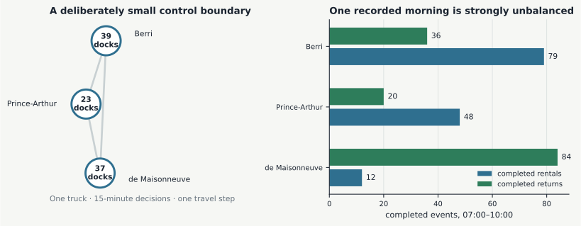
Figure 1:The three-station boundary contains 99 docks. Berri recorded 79 completed rentals and 36 returns, Prince-Arthur recorded 48 and 20, and de Maisonneuve recorded 12 and 84. The events come from the 2024 BIXI trip archive; capacities come from a station-information snapshot retrieved on 2 September 2026.
The simulation uses the station capacities recorded in a 2 September 2026 station-information snapshot for every run. Those values make the example reproducible, but they need not equal the capacities in service on 4 July 2024.
| station | ID | capacity |
|---|---|---|
| Berri / Cherrier | 173 | 39 |
| Prince-Arthur / St-Urbain | 404 | 23 |
| de Maisonneuve / Aylmer (ouest) | 68 | 37 |
Let be the number of bicycles at station , its capacity, and the truck inventory. A transfer is positive when the truck unloads bicycles at its current station and negative when it loads them. The post-transfer stock at the start of an interval is .
Attempted rentals and returns then arrive as a chronological event sequence. For event , let indicate a served rental and an accepted return. Their values depend on the stock immediately before the event:
If interval contains events, its inventory balance is
Relocation cancels when station and truck inventories are added. Customer trips can still change the total inside this three-station boundary because their other endpoint may lie elsewhere in the network.
The teaching plant begins with station inventories and an empty 16-bike truck at de Maisonneuve. Decisions occur every 15 minutes. A stop may transfer at most eight bicycles, and travel between any two of the three stations consumes one decision interval. At a common station and timestamp, the simulator processes returns before rentals. It records lost rentals and rejected returns instead of silently clipping attempted events.
Three controllers receive the same event trace. The first never relocates a bike. The second freezes a schedule computed before 07:00 from mean completed trip counts. The third reevaluates a deterministic, hand-written rule every 15 minutes using the observed inventories. It does not solve an optimization problem at each decision time. Here feedback means that the current observation enters the rule; it does not imply optimization or learning.
Both active controllers use the remaining-horizon target
The function limits to the interval . Thus the target begins at half capacity, shifts upward when future departures are expected to exceed arrivals, and remains between 20 and 80 percent of station capacity. Here and are the mean numbers of completed departures and arrivals at station during 15-minute interval across the 43 calibration dates. Define the current deficit and surplus relative to the target by
The positive-part operator makes deficit and surplus nonnegative. At most one is positive for a given station. The rule first decides what to transfer at the truck’s current station. If the truck carries bicycles and the local deficit is at least two, it unloads. If the local surplus is at least two and the other stations have a combined deficit of at least two, it loads. Transfer size is capped by the eight-bike stop limit, truck capacity, available bicycles, open docks, and the relevant surplus or deficit. If the truck still carries bicycles after the transfer, it drives toward the other station with the largest ratio . If it is empty, and both a deficit and a surplus of at least two remain, it drives toward the other station with the largest ratio . Distance breaks ties. Finally, when the truck carries leftover bicycles but the total modeled deficit is below two, it returns as many as possible at its current station rather than keeping them unavailable to customers.
The frozen schedule is produced before 07:00 by applying this same heuristic to one deterministic mean-flow trajectory. It then keeps those actions unchanged. That calculation makes it an open-loop plan, not a second online optimizer. In the resulting schedule, the truck waits at de Maisonneuve, loads three bicycles at 07:45, travels to Prince-Arthur, and unloads them at 08:00. The feedback controller instead recomputes the rule from each newly observed inventory.
For the stochastic comparison, let be the number of completed events of type at station in interval on calibration date . The empirical rate and simulated count are
The Poisson distribution is a count model whose mean here is . The count draws are independent across stations, intervals, and event types. Conditional on , the simulator places the event times independently and uniformly inside interval . It treats these events as potential attempts and accepts or rejects each one using the inventory equations above. Thus the model turns rates estimated from completed trips into attempted-event rates. This is a declared modeling assumption: the public archive does not identify demand that was censored by an empty or full station.
For each seed from 0 through 511, all three controllers receive the same sampled event trace. This common-random-number design compares their decisions under the same demand realization. A separate paired-pulse condition appends eight rental attempts at Prince-Arthur at 07:47 and eight return attempts at de Maisonneuve at 07:57 to every trace. These additions are fixed, not extra Poisson draws, and each succeeds only when inventory or dock space permits. The feedback rule first uses their inventory consequences at the 08:00 decision. The frozen controller receives the new observation but ignores it and executes the action selected before 07:00.
The recorded comparison below uses the same event trace for every controller. The map, station fills, truck motion, and service failures come from committed Python trajectories. Controller selection and the playhead only seek through those records; they do not recompute the plant in the browser.
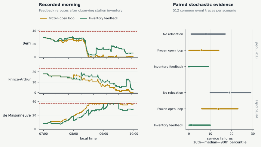
Figure 2:Static trajectories and paired stochastic evidence from the same Python experiment. The online book adds controller selection, playback, stepping, and scrubbing.
| controller | mean failures, rate model | mean failures, paired pulse |
|---|---|---|
| No relocation | 8.78 | 19.30 |
| Frozen open loop | 6.21 | 14.78 |
| Inventory feedback | 3.06 | 3.60 |
On the nominal traces, feedback lowers mean failures from 6.21 to 3.06 relative to the frozen plan. The frozen plan moves a median 6 bicycles over 0.85 km. Feedback moves a median 20 bicycles over 4.05 km under the rate model and 33 bicycles over 5.09 km under the paired pulse. The service gain therefore comes with a visible relocation cost.
Values are means over 512 common-random-number event traces. They describe the teaching simulator calibrated from completed trips, not measured failures in BIXI operations.
Feedback reduces service failures in this model, but it does more relocation work. These are outcomes of the stated simulator, not measurements of service failures or estimates of a causal effect in BIXI operations. The public archive omits unsuccessful attempts, historical inventories, and operator truck movements. The selected morning was chosen after inspection because its imbalance is easy to see; it is not an unbiased evaluation sample BIXI Montréal (2024)Ville de Montréal (2026)Hulot et al. (2018).
Inspect the BIXI transition and feedback rule
1 2 3 4 5 6 7 8 9 10 11 12 13 14 15 16 17 18 19 20 21 22 23 24 25 26 27 28 29 30 31 32 33 34 35 36 37 38 39 40 41 42 43 44 45 46 47 48 49 50 51 52 53 54 55 56 57 58 59 60 61 62 63 64 65 66 67 68 69 70 71 72 73 74 75 76 77 78 79 80 81 82 83 84 85 86 87 88 89 90 91 92 93 94 95 96 97 98 99 100 101 102 103 104 105 106 107 108 109class InventoryFeedbackController: name: ControllerName = "feedback" def __init__(self, scenario: BixiScenario, profile: CompletedEventProfile): scenario.validate() profile.validate(len(scenario.stations)) if profile.decision_count != scenario.decision_count: raise ValueError("profile and scenario horizons differ") self.scenario = scenario self.profile = profile def target_inventory(self, decision_index: int) -> np.ndarray: remaining_net_rentals = np.sum( self.profile.completed_starts[decision_index:] - self.profile.completed_ends[decision_index:], axis=0, ) capacities = self.scenario.capacities return np.clip( 0.5 * capacities + remaining_net_rentals, 0.2 * capacities, 0.8 * capacities, ) def __call__(self, observation: BixiObservation) -> BixiAction: scenario = self.scenario x = np.asarray(observation.station_inventory, dtype=float) b = int(observation.truck_inventory) location = int(observation.truck_station) target = self.target_inventory(observation.decision_index) deficit = np.maximum(target - x, 0.0) surplus = np.maximum(x - target, 0.0) transfer = 0 if b > 0 and deficit[location] >= 2.0: transfer = int( min( scenario.transfer_limit, b, np.ceil(deficit[location]), scenario.capacities[location] - x[location], ) ) else: remote = np.arange(len(scenario.stations)) != location remote_deficit = float(np.sum(deficit[remote])) if ( surplus[location] >= 2.0 and b < scenario.truck_capacity and remote_deficit >= 2.0 ): load = int( min( scenario.transfer_limit, scenario.truck_capacity - b, np.floor(surplus[location]), np.ceil(remote_deficit), x[location], ) ) transfer = -load elif ( b > 0 and float(np.sum(deficit)) < 2.0 and scenario.capacities[location] - x[location] >= 1.0 ): # Bikes left on the truck are unavailable to customers. Return # them when no modeled target deficit remains. transfer = int( min( scenario.transfer_limit, b, scenario.capacities[location] - x[location], ) ) x_after = x.copy() x_after[location] += transfer b_after = b - transfer deficit_after = np.maximum(target - x_after, 0.0) surplus_after = np.maximum(x_after - target, 0.0) if b_after > 0 and float(np.max(deficit_after)) >= 2.0: score = deficit_after / scenario.capacities elif ( b_after == 0 and float(np.max(deficit_after)) >= 2.0 and float(np.max(surplus_after)) >= 2.0 ): score = surplus_after / scenario.capacities else: return BixiAction(transfer=transfer, destination=location) score = score.copy() score[location] = -np.inf best = float(np.max(score)) if best <= 0.0: destination = location else: tied = np.flatnonzero(np.isclose(score, best)) destination = min( (int(index) for index in tied), key=lambda index: ( scenario.distance_km[location, index], index, ), ) return BixiAction(transfer=transfer, destination=destination)
1 2 3 4 5 6 7 8 9 10 11 12 13 14 15 16 17 18 19 20 21 22 23 24 25 26 27 28 29 30 31 32 33 34 35 36 37 38 39 40 41 42 43 44 45 46 47 48 49 50 51 52 53 54 55 56 57 58 59 60 61 62 63 64 65 66 67 68 69 70 71 72 73 74 75 76 77 78 79 80 81 82 83 84 85 86 87 88 89 90 91 92 93 94 95 96 97 98 99 100 101 102 103 104 105 106 107 108 109 110 111 112 113 114 115 116 117 118 119 120 121 122 123 124 125 126 127 128 129 130 131 132 133 134 135 136 137 138 139 140 141 142 143 144 145 146 147 148 149 150 151 152 153 154 155 156 157 158 159 160 161 162 163 164 165 166 167 168 169 170 171 172 173 174def simulate( scenario: BixiScenario, trace: EventTrace, controller: Controller, ) -> BixiTrajectory: scenario.validate() trace.validate(scenario) inventory = scenario.initial_inventory.astype(float).copy() truck_inventory = scenario.initial_truck_inventory truck_station = scenario.initial_truck_station period = scenario.control_period_minutes decisions = scenario.decision_count checkpoints = [inventory.copy()] truck_checkpoints = [truck_inventory] location_checkpoints = [truck_station] requested_transfers: list[int] = [] realized_transfers: list[int] = [] destinations: list[int] = [] cumulative_lost = [0] cumulative_rejected = [0] cumulative_moved = [0] cumulative_distance = [0.0] event_times: list[float] = [] event_stations: list[int] = [] event_kinds: list[EventKind] = [] event_accepted: list[bool] = [] event_inventory_after: list[float] = [] history_times = [0.0] history_inventory = [inventory.copy()] history_truck = [truck_inventory] attempted_rentals = served_rentals = 0 attempted_returns = accepted_returns = 0 lost_rentals = rejected_returns = 0 bikes_moved = unrealized_transfer_bikes = 0 distance_km = 0.0 event_index = 0 for decision in range(decisions): start = float(decision * period) stop = float((decision + 1) * period) observation = BixiObservation( decision_index=decision, time_minutes=start, station_inventory=inventory.copy(), truck_inventory=truck_inventory, truck_station=truck_station, ) action = controller(observation) previous_station = truck_station inventory, truck_inventory, truck_station, realized = _apply_action( scenario, inventory, truck_inventory, truck_station, action, ) requested_transfers.append(int(action.transfer)) realized_transfers.append(realized) destinations.append(truck_station) unrealized_transfer_bikes += abs(int(action.transfer) - realized) bikes_moved += abs(realized) distance_km += float(scenario.distance_km[previous_station, truck_station]) history_times.append(start) history_inventory.append(inventory.copy()) history_truck.append(truck_inventory) while event_index < len(trace.events): event = trace.events[event_index] if event.time_minutes >= stop: break station = event.station_index accepted = False if event.kind == "rental": attempted_rentals += 1 if inventory[station] >= 1.0: inventory[station] -= 1.0 served_rentals += 1 accepted = True else: lost_rentals += 1 else: attempted_returns += 1 if inventory[station] < scenario.capacities[station]: inventory[station] += 1.0 accepted_returns += 1 accepted = True else: rejected_returns += 1 event_times.append(event.time_minutes) event_stations.append(station) event_kinds.append(event.kind) event_accepted.append(accepted) event_inventory_after.append(float(inventory[station])) history_times.append(event.time_minutes) history_inventory.append(inventory.copy()) history_truck.append(truck_inventory) event_index += 1 checkpoints.append(inventory.copy()) truck_checkpoints.append(truck_inventory) location_checkpoints.append(truck_station) cumulative_lost.append(lost_rentals) cumulative_rejected.append(rejected_returns) cumulative_moved.append(bikes_moved) cumulative_distance.append(distance_km) if event_index != len(trace.events): raise RuntimeError("simulation ended before all events were processed") if np.any(inventory < 0.0) or np.any(inventory > scenario.capacities): raise RuntimeError("simulation violated station bounds") if not 0 <= truck_inventory <= scenario.truck_capacity: raise RuntimeError("simulation violated the truck bound") initial_total = float(np.sum(scenario.initial_inventory)) + scenario.initial_truck_inventory expected_total = initial_total + accepted_returns - served_rentals actual_total = float(np.sum(inventory)) + truck_inventory if not np.isclose(expected_total, actual_total): raise RuntimeError("inventory conservation check failed") terminal_imbalance = float( np.sum(np.abs(inventory - 0.5 * scenario.capacities)) + truck_inventory ) service_failures = lost_rentals + rejected_returns objective = float( scenario.failure_weight * service_failures + scenario.bike_moved_weight * bikes_moved + scenario.distance_weight * distance_km + scenario.terminal_imbalance_weight * terminal_imbalance ) metrics = BixiMetrics( attempted_rentals=attempted_rentals, served_rentals=served_rentals, attempted_returns=attempted_returns, accepted_returns=accepted_returns, lost_rentals=lost_rentals, rejected_returns=rejected_returns, service_failures=service_failures, bikes_moved=bikes_moved, truck_distance_km=distance_km, unrealized_transfer_bikes=unrealized_transfer_bikes, terminal_imbalance=terminal_imbalance, terminal_truck_inventory=truck_inventory, objective=objective, ) return BixiTrajectory( controller_name=controller.name, source_label=trace.source_label, checkpoint_time_minutes=np.arange(decisions + 1, dtype=float) * period, station_inventory=np.asarray(checkpoints, dtype=float), truck_inventory=np.asarray(truck_checkpoints, dtype=int), truck_station=np.asarray(location_checkpoints, dtype=int), requested_transfer=np.asarray(requested_transfers, dtype=int), realized_transfer=np.asarray(realized_transfers, dtype=int), destination=np.asarray(destinations, dtype=int), cumulative_lost_rentals=np.asarray(cumulative_lost, dtype=int), cumulative_rejected_returns=np.asarray(cumulative_rejected, dtype=int), cumulative_bikes_moved=np.asarray(cumulative_moved, dtype=int), cumulative_distance_km=np.asarray(cumulative_distance, dtype=float), event_time_minutes=np.asarray(event_times, dtype=float), event_station=np.asarray(event_stations, dtype=int), event_kind=tuple(event_kinds), event_accepted=np.asarray(event_accepted, dtype=bool), event_inventory_after=np.asarray(event_inventory_after, dtype=float), history_time_minutes=np.asarray(history_times, dtype=float), history_station_inventory=np.asarray(history_inventory, dtype=float), history_truck_inventory=np.asarray(history_truck, dtype=int), metrics=metrics, )
The BIXI simulator supplies station and truck inventories directly to the feedback controller. Physical sensors often provide only indirect, noisy measurements of the state.
Partial Observability
A transition kernel describes uncertainty in the state itself. What changes when the controller receives only a noisy or ambiguous function of that state?
The BIXI controller receives the modeled inventories directly. Many controllers instead receive sensor readings that contain only partial or noisy information about the predictive state. An observation model relates the hidden state to the available measurement:
Here is the distribution assigned to measurement noise. For a linear Gaussian sensor, with . A controller based only on may lose information needed to predict future transitions. Under a known model, the posterior belief
assigns a probability to each set of possible hidden states. This belief is an information state: it retains the predictive content of the observation history in a form that can be updated after each action and measurement. A point estimate is often cheaper to use, but it may discard uncertainty that affects future decisions.
Camera Stabilization under Partial Observation
Picture a camera on a one-axis gimbal attached to a moving vehicle. The motor tries to keep the horizon level. A tap can rotate the camera, and a sideways acceleration of the vehicle can disturb its sensors even when the camera itself does not rotate. The controller must infer what happened from an inertial measurement unit rather than from the true angle.
The simulated hidden state is
where is the camera angle in radians, is its angular velocity in radians per second, and is an offset in the gyroscope reading, also in radians per second. The camera is balanced about the gimbal axis, so gravity does not create a rotational torque in this model. Its one-axis torque balance is
Here is the camera’s moment of inertia about the gimbal axis, measured in . A larger means that the same torque produces less angular acceleration. The motor torque and external torque are measured in , and is a viscous rotational-damping coefficient measured in . The bound represents the motor’s torque limit.
The bias belongs to the sensor, not to the mechanical plant. If the camera is motionless but degrees per second, the gyroscope reading remains centered near 0.8 degrees per second instead of zero. This persistent offset is different from the small, rapid fluctuations that vary independently from one measurement to the next.
Real sensor errors depend on temperature, calibration, and hardware. For this ten-second simulation, a random walk provides a simple model of an offset that persists but can drift El-Sheimy et al. (2008):
Conditional on , the next bias has mean and its change has standard deviation . Nothing in the model pulls the bias back to zero. Here degrees per second and , so the standard deviation of one bias change is only 0.002 degrees per second at the -second sensor period. The chosen random walk therefore changes slowly relative to the sample-to-sample measurement noise. It is a reproducible teaching model, not a claim that every gyroscope drifts in exactly this way.
The gyroscope measures angular velocity with both the persistent bias and sample-to-sample measurement noise:
Integrating these readings turns a rate estimate into an angle estimate. Over seconds, an approximately constant bias contributes roughly to that estimated angle. A camera that is actually motionless therefore acquires about eight degrees of estimated rotation after ten seconds when an uncorrected 0.8-degree-per-second bias is integrated. Zero-mean measurement noise tends to fluctuate in both directions; the persistent offset accumulates in one direction.
The accelerometer creates a different ambiguity. It measures specific force, the force per unit mass sensed by its internal proof mass, rather than reporting a camera angle directly. When the vehicle is stationary or moves at constant velocity, the support force opposing gravity supplies a vertical reference. A sideways vehicle acceleration changes the same sensor reading and can therefore look like camera tilt Android Developers (2026).
The simulation keeps only the two axes in the plane of rotation. Its accelerometer model is
The vector contains the vehicle’s sideways acceleration and the gravity reference in world coordinates. The rotation expresses that vector along the camera-mounted sensor axes, and adds instantaneous measurement noise. If sideways acceleration and measurement noise are both zero, the direction of this vector determines . With sideways acceleration, the angle inferred from the same two components becomes
For example, adds an apparent tilt of about 17 degrees. A level camera on a vehicle accelerating sideways can then produce the same accelerometer direction as a tilted camera on a stationary base. This is the partial-observation problem: the sensor reading alone does not identify which hidden situation occurred.
The two sensors fail on different time scales. The accelerometer gives a stable long-run reference when vehicle translation is mild, but a lateral acceleration corrupts it immediately. The gyroscope tracks rapid rotations without confusing them with translation, but integrating an unknown bias produces long-run drift. A complementary observer is a recursive state estimator that combines these two time scales. It uses the gyroscope for rapid changes, the accelerometer for slow angle correction, and the persistent disagreement between them to estimate gyroscope bias Mahony et al. (2008).
The comparison below changes only the estimator. One controller uses the accelerometer direction as its angle estimate, one integrates the raw gyroscope, and one uses the complementary observer. Every run receives the same mechanical plant, noise realization, disturbances, torque limit, and feedback law:
The function limits the requested motor torque to the interval . The simulated plant uses , , one-millisecond mechanical integration, and ten-millisecond sensing and control. The ten-second sensor trace is generated once with seed 11 and then supplied unchanged to every estimator.
All three runs start with the camera tilted by eight degrees. A tap from 1.50 to 1.62 seconds physically rotates the camera, so both inertial sensors should help the controller respond. From 4.0 to 4.6 seconds, the base instead accelerates sideways at up to . That event changes the accelerometer reading without directly rotating the balanced camera. The final quiet interval exposes the angle error produced by integrating the biased gyroscope.
The replay displays curves only up to the current playhead. Its metrics use the hidden simulated angle, which is available to the experiment but not to the controllers.
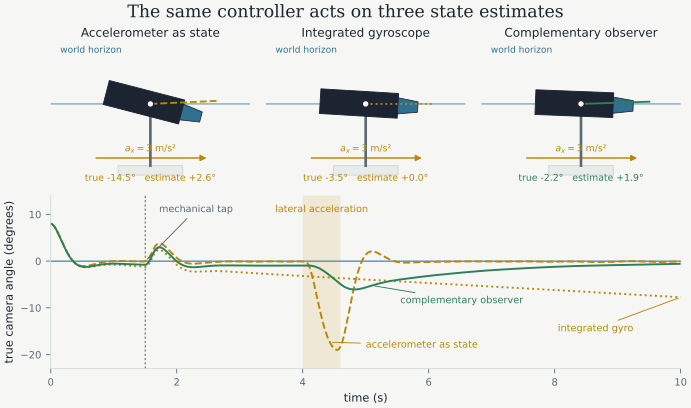
Figure 3:Static snapshots and complete trajectories from the same Python experiment. The online book adds playback, stepping, and scrubbing.
| state estimate supplied to the controller | RMS angle | peak during translation | final absolute error |
|---|---|---|---|
| Accelerometer as state | 3.86 degrees | 19.00 degrees | 0.08 degrees |
| Integrated gyroscope | 4.60 degrees | 4.31 degrees | 7.73 degrees |
| Complementary observer | 2.43 degrees | 6.07 degrees | 0.58 degrees |
The results follow the two failure mechanisms. The accelerometer-only estimate reacts strongly to the translation pulse. The integrated-gyroscope estimate largely ignores that pulse but drifts during the quiet interval. The complementary observer reduces both errors by using the accelerometer as a slow correction to the gyroscope-based angle. Sustained unknown translation can still be mistaken for tilt. These are results from a transparent teaching simulation, not measured performance of a commercial gimbal.
The same distinction appears in adaptive optics: local wavefront slopes are sensor observations, while the reconstructed phase is the state used for control.
Inspect the sampled plant, sensors, estimator, and controller
1 2 3 4 5 6 7 8 9 10 11 12 13 14 15 16 17 18 19 20 21 22 23 24 25 26 27 28 29 30 31 32 33 34 35 36 37 38 39 40 41 42 43 44 45 46 47 48 49 50 51 52 53 54 55 56 57 58 59 60 61 62 63 64 65 66 67 68 69 70 71 72 73 74 75 76 77 78 79 80 81 82 83 84 85 86 87 88 89 90 91 92 93 94 95 96 97 98 99 100def sample_observation( state: np.ndarray, gyro_bias_rad_s: float, lateral_acceleration_mps2: float, gyro_noise_rad_s: float, accelerometer_noise_mps2: np.ndarray, parameters: GimbalParameters, ) -> GimbalObservation: """Sample a gyro and two-axis accelerometer in the camera frame.""" angle_rad, angular_velocity_rad_s = np.asarray(state, dtype=float) noise = np.asarray(accelerometer_noise_mps2, dtype=float) if noise.shape != (2,): raise ValueError("accelerometer_noise_mps2 must have shape (2,)") cosine = np.cos(angle_rad) sine = np.sin(angle_rad) accelerometer_x = ( cosine * lateral_acceleration_mps2 + sine * parameters.gravity_mps2 + noise[0] ) accelerometer_y = ( -sine * lateral_acceleration_mps2 + cosine * parameters.gravity_mps2 + noise[1] ) return GimbalObservation( gyro_rad_s=float(angular_velocity_rad_s + gyro_bias_rad_s + gyro_noise_rad_s), accelerometer_x_mps2=float(accelerometer_x), accelerometer_y_mps2=float(accelerometer_y), ) def update_estimator( estimator: EstimatorKind, memory: EstimatorMemory | None, observation: GimbalObservation, parameters: GimbalParameters, scenario: GimbalScenario, ) -> tuple[EstimatorMemory, np.ndarray]: """Update one transparent attitude estimator and return ``[angle, rate, bias]``.""" accelerometer_angle = observation.accelerometer_angle_rad if memory is None: memory = EstimatorMemory(accelerometer_angle, 0.0) return memory, np.array( [accelerometer_angle, observation.gyro_rad_s, 0.0], dtype=float ) if estimator == "accelerometer": updated = EstimatorMemory(accelerometer_angle, 0.0) estimate = np.array( [accelerometer_angle, observation.gyro_rad_s, 0.0], dtype=float ) elif estimator == "gyro": angle = float( wrap_angle(memory.angle_rad + scenario.sensor_period_s * observation.gyro_rad_s) ) updated = EstimatorMemory(angle, 0.0) estimate = np.array([angle, observation.gyro_rad_s, 0.0], dtype=float) elif estimator == "complementary": innovation = float(wrap_angle(accelerometer_angle - memory.angle_rad)) angle = float( wrap_angle( memory.angle_rad + scenario.sensor_period_s * ( observation.gyro_rad_s - memory.bias_rad_s + parameters.observer_angle_gain_per_s * innovation ) ) ) bias = float( memory.bias_rad_s - parameters.observer_bias_gain_per_s2 * scenario.sensor_period_s * innovation ) updated = EstimatorMemory(angle, bias) estimate = np.array( [angle, observation.gyro_rad_s - bias, bias], dtype=float ) else: raise ValueError(f"unknown estimator: {estimator}") return updated, estimate def saturated_pd(estimate: np.ndarray, parameters: GimbalParameters) -> float: """Apply the common saturated feedback law to an estimated state.""" angle_rad, angular_velocity_rad_s = np.asarray(estimate, dtype=float)[:2] requested = -( parameters.controller_kp_nm_per_rad * angle_rad + parameters.controller_kd_nm_s_per_rad * angular_velocity_rad_s ) return float( np.clip(requested, -parameters.torque_limit_nm, parameters.torque_limit_nm) )
State, action, disturbance, and observation equations describe the model’s semantics. An algorithm still needs a computational way to use that model. The next distinction concerns which operations the model exposes: formulas and derivatives, reset-and-step simulation, fixed logged transitions, or new online interaction.
Summary and Outlook
Transition kernels separate the action selected by the decision maker from the disturbance that selects a realized successor. Observation models add a second separation: the state supports prediction, while the measurement supplies only the information available for choosing the next action.
These equations specify what a model means, but they do not specify how an algorithm may use it. Can the algorithm differentiate the transition, reset a simulator, resample a state, or only inspect logged transitions? Model interfaces and learned components make those operations explicit.
Exercises
Solution to Exercise 1
Since and ,
Customer trips may later cross the three-station boundary and change that total. At 08:00, feedback observes the inventories produced by the unexpected Prince-Arthur rentals and de Maisonneuve returns, so it can alter its transfer or route. The frozen schedule was fixed from information available before 07:00 and has no rule for using the new observation.
Solution to Exercise 2
Both
produce an apparent tilt of . The gyroscope measures angular rate plus bias, which helps distinguish a rapid rotation from a translational pulse. An unknown gyro bias still accumulates as angle error, and sustained unknown translation remains confounded with gravity in the accelerometer.
Solution to Exercise 3
Solution to Exercise 4
Two request sets can have equal queue counts and cache occupancy but different remaining output lengths. Their completion times and cache releases therefore have different conditional distributions. A full state can retain every request’s remaining work. When that work is hidden, the complete observation history is sufficient in principle, and a posterior distribution over the request-level state is a compact information state under a known model.
Solution to Exercise 5
(a) The boundary contains the two queues, four workers, and their power-relevant operation. A full state contains the queued jobs, every active job’s worker and remaining processing time, the worker modes, and any variable needed to predict power. The stated observation contains the two queue counts, busy-worker count, worker modes, and measured power. The action is the active-worker count and queue priority. Arrivals and unobserved job requirements are disturbances. The stage cost combines waiting and energy, and the power cap is a hard constraint. Time is discrete in one-minute steps over 60 decisions.
(b) Equal counts can hide different remaining workloads and therefore different completion distributions. The full state just described is Markov under the declared job model. The complete observation-action history is available to the dispatcher; under a known stochastic model, its posterior over hidden job states is a more compact information state.
(c) A stochastic transition kernel is the natural representation because jobs arrive at random times and hidden processing requirements make completions uncertain. A deterministic function remains possible only after the relevant noise realizations are supplied as additional inputs.
(d) The fixed schedule selects all 60 actions from initial information. A feedback policy may change the active-worker count or priority after observing new queue counts, busy-worker status, modes, or power.
(e) Those data supply a logged-transition interface under one behavior schedule. It cannot directly answer how actions absent from that log would change queues or power, so evaluating a new feedback policy requires coverage and identification assumptions or a separate transition model.
Solution to Exercise 6
(a) The augmented latent state is , where counts hard problems already used. The observation is correctness and response time, and the action is difficulty. The model has a stochastic mastery transition and a stochastic observation map. The terminal objective is , with as a hard constraint. The horizon contains 20 actions. The available model is a generative reset-and-sample simulator.
(b) The latest answer alone generally loses information from earlier rounds. The complete history is sufficient but grows with time. Under the stated conditional relationships, the posterior , augmented by and , is a Markov information state.
(c) Without assigning numbers, the structure is
with a feasible feedback policy that excludes the hard action once .
(d) An open-loop sequence fixes all 20 difficulties before any answers are seen. A feedback sequence selects the next difficulty after updating the mastery posterior from correctness and response time, while retaining the remaining hard-problem budget.
(e) The simulator directly supports arbitrary one-step samples and Monte Carlo rollouts from chosen latent states and actions. Exact probabilities, analytic derivatives, or symbolic local equations require an additional interface.
- BIXI Montréal. (2024). Open Data: Trip History and Station Status. https://bixi.com/en/open-data/
- Ville de Montréal. (2026). BIXI Trip History. Montréal open-data catalogue. https://donnees.montreal.ca/dataset/bixi-historique-des-deplacements
- Hulot, P., Aloise, D., & Jena, S. D. (2018). Towards Station-Level Demand Prediction for Effective Rebalancing in Bike-Sharing Systems. Proceedings of the 24th ACM SIGKDD International Conference on Knowledge Discovery and Data Mining, 378–386. 10.1145/3219819.3219873
- El-Sheimy, N., Hou, H., & Niu, X. (2008). Analysis and Modeling of Inertial Sensors Using Allan Variance. IEEE Transactions on Instrumentation and Measurement, 57(1), 140–149. 10.1109/TIM.2007.908635
- Android Developers. (2026). Motion Sensors. https://developer.android.com/develop/sensors-and-location/sensors/sensors_motion
- Mahony, R., Hamel, T., & Pflimlin, J.-M. (2008). Nonlinear Complementary Filters on the Special Orthogonal Group. IEEE Transactions on Automatic Control, 53(5), 1203–1218. 10.1109/TAC.2008.923738