Stochastic dynamics and observation models specify the law of the next state and the information returned to the controller. Which of those mathematical objects can an algorithm actually evaluate, differentiate, resample, or learn from recorded data?
Two models may generate the same nominal trajectory while exposing different operations to an algorithm. Access to equations, derivatives, resets, and new interactions determines what can be computed. The interface therefore matters independently of the model’s physical fidelity: knowing that a transition exists is different from being able to differentiate it, resample it, or query it under a new action.
| available interface | operations it supports directly | methods developed later |
|---|---|---|
| equations and derivatives | evaluate local dynamics, linearize, differentiate constraints | direct transcription, LQR, gradient-based MPC |
| one-step transition function | reset and advance from chosen state-action pairs | shooting, simulation-based MPC, model-based dynamic programming |
| generative simulator | sample trajectories without inspecting internal equations | Monte Carlo estimation, derivative-free search, policy learning |
| logged transitions | fit or evaluate models on the recorded distribution | system identification, fitted value and Q methods, offline evaluation |
| interactive environment and objective | collect new transitions under chosen actions | online reinforcement learning |
The rows are not mutually exclusive. A simulator may be differentiable, an explicit model may contain unknown parameters, and logged data can be used to fit a new one-step model. The table records the information supplied to the algorithm, not the origin or fidelity of the model.
A program is a model when its execution defines state transitions. MuJoCo, for example, combines rigid-body equations, contact detection, constraint forces, sensors, and rendering behind a reset-and-step interface. A user can query that interface without possessing a practical expression for its complete local transition function. A discrete-event simulator also defines a transition model, although its clock advances from one asynchronous event to the next.
Calling a method model-free specifies which transition information its updates can use. In this book, a model-free update receives sampled experience rather than direct access to the transition function, transition probabilities, or their derivatives. An online method may choose an action and observe the resulting transition. An offline method is restricted to the transitions in its log. Neither can directly request the exact outcome distribution for an untried action at the same state. Both still require a declared observation, action set, reward, sampling process, and assumptions connecting the available samples to deployment.
Inference Serving as a Controlled System
Inference serving contains several modeling choices within one boundary. It combines conserved work and cache balances with profiled performance maps, has both request-level and aggregate states, and can be accessed through equations, simulation, logged traces, or a live process. The control objective is to schedule work and choose hardware settings while respecting latency, memory, power, and thermal limits.
An inference server receives prompts at irregular times and generates one response for each request. A decoder-only language model processes a request in two phases. The prefill phase processes the prompt in parallel and creates the first output token. The decode phase generates the remaining tokens one iteration at a time. Long prefills can delay the short decode iterations of requests already in progress. Iteration-level scheduling and chunked prefill are production approaches to controlling this interaction Yu et al. (2022)Agrawal et al. (2024). The teaching simulator below uses a reduced interleaving rule rather than reproducing either serving system.
Boundary, State, and Action
The system boundary surrounds one GPU and its serving process. The language model and inference engine lie inside the boundary. Request arrivals and ambient thermal conditions enter from outside it.
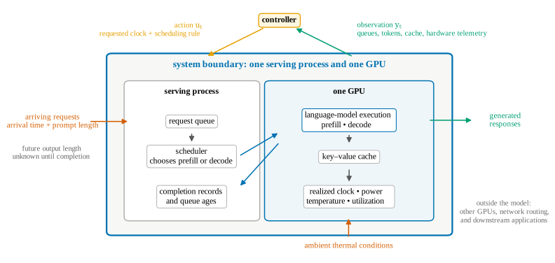
Figure 1:The boundary contains the request queue, scheduler, language-model execution, key-value cache, and GPU hardware state. The controller observes queue and cache state, completed work, power, temperature, and realized clock; it chooses a requested clock and scheduling rule. Arrivals are disturbances, and a request’s eventual output length remains hidden until that request completes. Other GPUs, network routing, and downstream applications remain outside this model.
This fixed serving boundary is available through four of the interfaces above. Token, cache, and thermal balances provide equations. The profile-based event simulator can be reset and run under chosen clock and scheduling actions. Logged traces and profile records contain only the states and actions that were recorded, so they cannot directly answer counterfactual questions outside that coverage. A live Qwen/vLLM process accepts new requests and chosen clock settings, producing new transition samples. Several interfaces may coexist; their available operations differ even though the serving process does not.
The full request-level simulator state records each request’s phase, age, remaining prompt work, generated tokens, eventual output length, and cache allocation. The eventual output length is part of the simulator’s hidden state but is not revealed to the controller. At a one-second control interval, the reduced control model uses the aggregate state
where is queued prefill work and is unfinished decode work. The quantity is key-value-cache occupancy; this cache stores intermediate attention representations so that previously processed tokens need not be recomputed at each decode step. The remaining variables are GPU temperature and realized graphics clock , the hardware frequency that determines how quickly GPU work can proceed. This vector is a state of the reduced model, but it is not a Markov description of every request-level trajectory. The control
combines a requested clock with a scheduling rule . The scheduler decides which phase receives each service step and how much prefill work may be processed before returning to active decodes. The clock request changes the rate and energy cost of that work. Hardware may realize a lower clock under a power or thermal limit, so and are distinct variables NVIDIA Corporation (2026).
Request arrivals form the disturbance. An arrival supplies its time and prompt length, but its eventual output length remains unknown to the controller until the end-of-sequence token arrives. The observation contains queue ages, completed prompt and output tokens, cache use, power, temperature, and realized clock. This information pattern prevents a controller from scheduling with the future length recorded in an evaluation trace.
Conservation and Calibrated Maps
The aggregate balances expose structure that does not have to be learned. If prompt tokens arrive, prompt tokens are processed, requests finish prefill, and decode tokens are produced, then
The term denotes the still-unknown output work associated with newly admitted decode requests. The request-level simulator makes this work available only as tokens complete. It tracks continuous prompt and generated-token occupancy, including partial prefills, together with a fixed per-request reserve. That occupancy is released when a request completes. This aggregate accounting preserves the modeled cache balance, but it does not reproduce a serving engine’s block allocator. An aggregate thermal balance has the form
Here is ambient temperature, is effective thermal capacitance, and is thermal resistance to the surroundings. The power map adds heat, while removes heat when the GPU is warmer than its environment.
Token and cache conservation determine the form of the transition. Measurements are still needed for the service-rate map, the power map , and the thermal parameters. The profiling protocol targets Qwen2.5-7B-Instruct served by vLLM on an NVIDIA L4 Qwen Team (2025)Kwon et al. (2023). Its intended hardware profile spans five requested clock levels, several prompt lengths, and three concurrency levels, meaning three different numbers of requests served at the same time. The book build reads a committed profile and never starts a model server. Its manifest states whether the maps come from completed L4 measurements or a pre-measurement engineering surrogate, and every rendered result displays that provenance.
Batch Size Changes the Service Map
The recorded 64.8 W L4 profile shows why a service map must retain concurrency. At a requested 2,040 MHz with a 1,024-token prompt, aggregate decode throughput rises from 17.5 generated tokens per second for one request to 105.6 for eight concurrent requests. Aggregate prefill throughput changes much less across these batch sizes. Pooling the measurements into one rate per clock loses this difference and can give a controller the wrong prediction of queue drainage.
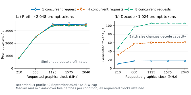
Figure 2:Batch size changes decode capacity in the recorded 2 September 2026 L4 profile at a 64.8 W cap. Each point is the median of five concurrent batches; whiskers show their minimum and maximum. Prompt length is fixed within each panel. All five requested clocks are retained, including the throughput plateau above 1,125 MHz.
The plateau also motivates a fixed moderate-clock baseline. A feedback controller can lower energy relative to the maximum clock without improving on a well-chosen constant clock. The live experiment therefore selects a constant clock on development requests before comparing it with the governor and MPC on fresh requests. The current live experiment uses a 40 W cap and requires fresh service and idle power measurements at that cap. The 64.8 W curves remain historical evidence; the replay below retains the original reduced teaching model.
The live controller distinguishes requests awaiting their first output from requests already streaming. It estimates remaining output work from development request lengths and the tokens received so far, then fits its transition model on mixed-serving measurements. These observations preserve useful differences in the workload without exposing unfinished requests’ final lengths or assuming that the resulting state is fully Markov.
Download the phase, context, and concurrency calibration table (CSV)
A separate measured study now compares fixed clocks, GPU-managed graphics clocks, and a causal demand/phase heuristic under the configured 40 W setting. Across four held-out Azure request blocks, each repeated twice, fixed 660 MHz used 10.31% less telemetry-derived GPU energy than GPU-managed clocks; the adaptive heuristic used a further 0.77% less than fixed 660 MHz. All paired relative latency checks passed, but the candidate failed development qualification and all three methods missed the absolute time-to-first-token target on the shorter code block. These are exploratory observations, not established latency-qualified adaptive savings. The heuristic is separate from the governor and MPC, whose calibration remains incomplete. The measured study includes the five-clock screen, request-shape probes, observed clocks, and retained failures.
Read the completed study and paired results (PDF)
Workload and Scheduling Rule
The conservation equations specify how work moves through the server, but an experiment also needs a reproducible arrival process and a declared scheduler. The following settings define the recorded simulation. The revised live experiment instead measures mixed-serving capacity and freezes its latency targets from development requests before confirmation.
The simulated workload is a five-minute excerpt from the Azure 2023 code-generation trace, which records request times and input and output token counts Microsoft Azure (2023)Patel et al. (2024). Arrival times are dilated once to place maximum-clock utilization near 80 percent. This time dilation preserves request sizes and ordering while spreading arrivals over a longer interval. If is the isolated service time of all requests at the highest profiled clock divided by the original window length, the dilation and normalized arrivals are
The factor is at least one, so it can leave the trace unchanged or slow its arrivals; it never compresses them into a shorter interval.
All simulated controllers receive the same immutable requests after this transformation. The simulated time-to-first-token limit is twice the median baseline value for a 1,024-token prompt at concurrency one and the highest clock. The time-per-output-token limit is 1.5 times the corresponding median. These are reference levels for a controlled comparison, not service-level objectives claimed for production systems.
| quantity | recorded simulation setting |
|---|---|
| model | Qwen2.5-7B-Instruct, revision acbd96531cda22292a3ceaa67e984955d3965282 Qwen Team (2025) |
| inference engine | vLLM OpenAI server, version 0.28.0 vLLM Project (2026) |
| target accelerator | one NVIDIA L4 |
| clock profile | five requested graphics clocks; realized clock, power, utilization, and temperature retained |
| request trace | first five minutes for evaluation; first 20 requests for the animation |
| controller sampling | one second |
| service simulation | 0.1-second steps; decode priority or one prefill chunk first; unused prefill capacity may return to decode |
| output length | hidden from the controller until completion |
Within each one-second clock-control period, the scheduler gives each 0.1-second simulator step to decode or begins it with one prefill chunk. If that chunk finishes before the step’s service budget is exhausted, the remaining capacity returns to decode. When both phases have work, active decode receives alternating-step priority and strict priority under high cache pressure. The 512-token interleaved chunked-prefill rule specifies the teaching model’s action channel; it does not reproduce vLLM’s mixed-batch scheduler or Sarathi-Serve.
Recorded Replay and Scope
The first 20 requests form the recorded replay below. They move through arrival, interleaved 512-token prefill chunks, autoregressive decode, and completion. The plots report only the trajectory prefix reached by the playhead, and output length is hidden from the controller until each request completes. A provenance badge distinguishes a verified measured profile from a pre-measurement engineering surrogate.
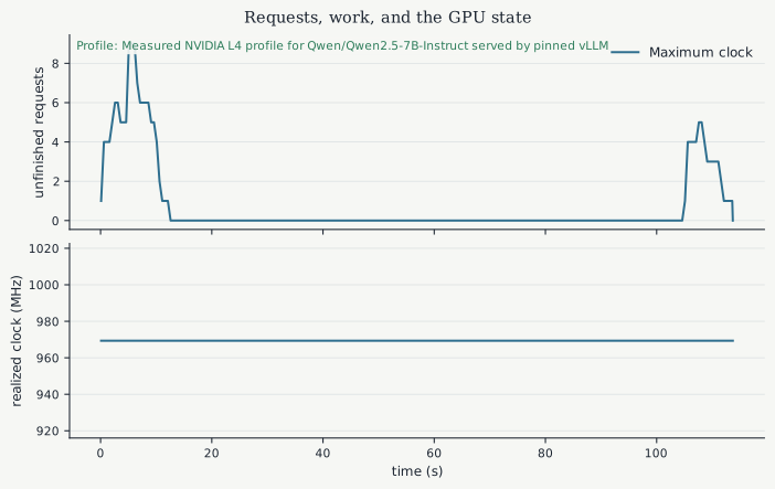
Figure 3:Static summary of unfinished requests and realized clock from the same request-level simulation. The online book provides playback, stepping, scrubbing, phase detail, and controller selection.
Conservation checks account for every request, processed token, and cache allocation. At the end of the committed replay, all 20 requests have completed, the prefill and decode queues are empty, and all modeled cache occupancy has been released. This establishes closure of the modeled flows. It does not show that the aggregate variables are Markov for the request-level plant, nor that the service-rate, power, or thermal maps are accurate. A provisional profile permits tests of the simulation and control software but does not supply empirical latency or energy evidence. In either case, the model does not cover every inference engine or GPU. Network transfer, host-side tokenization, multi-GPU communication, model-quality effects, and failures outside the serving process remain outside the boundary.
Inspect the request-level transition
1 2 3 4 5 6 7 8 9 10 11 12 13 14 15 16 17 18 19 20 21 22 23 24 25 26 27 28 29 30 31 32 33 34 35 36 37 38 39 40 41 42 43 44 45 46 47 48 49 50 51 52 53 54 55 56 57 58 59 60 61 62 63 64 65 66 67 68 69 70 71 72 73 74 75 76 77 78 79 80 81 82 83 84 85 86 87 88 89 90 91 92 93 94 95 96 97 98 99 100 101 102 103 104 105 106 107 108 109 110 111 112 113 114 115 116 117 118 119 120 121 122 123 124 125 126 127 128 129 130 131 132 133 134 135 136 137 138 139 140 141 142 143 144 145 146 147 148 149 150 151 152 153 154 155 156 157 158 159 160 161 162 163 164 165 166 167 168 169 170 171 172 173 174 175 176 177 178 179 180 181 182 183 184 185 186 187 188 189 190 191 192 193 194 195 196 197 198 199 200 201 202 203 204 205 206 207 208 209 210 211 212 213 214 215 216 217 218 219 220 221 222 223 224 225 226 227 228 229 230 231 232 233 234 235 236 237 238 239 240 241 242 243 244 245 246 247 248 249 250 251 252 253 254 255 256 257 258 259 260 261 262 263 264 265 266 267 268 269def simulate( workload: Sequence[Request], plant: ServingPlant, scheduler: Scheduler, clock_controller: ClockController, seed: int = 0, *, controller_name: str | None = None, scheduler_name: str | None = None, ) -> ServingResult: """Simulate one immutable workload under supplied feedback laws.""" del seed # The current plant is deterministic; the argument fixes the public API. plant.validate() requests = tuple(workload) if not requests: raise ValueError("workload must contain at least one request") for request in requests: request.validate() if len({request.request_id for request in requests}) != len(requests): raise ValueError("request identifiers must be unique") if any( right.arrival_time_s < left.arrival_time_s for left, right in zip(requests, requests[1:]) ): raise ValueError("workload must be sorted by arrival_time_s") runtime = [ _RuntimeRequest(request=request, prefill_remaining=float(request.prompt_tokens)) for request in requests ] pending_index = 0 prefill: list[_RuntimeRequest] = [] active: list[_RuntimeRequest] = [] completed: list[_RuntimeRequest] = [] temperature = plant.ambient_temperature_c previous_clock = plant.profile.minimum_realized_clock_mhz previous_power = plant.profile.power( "idle", plant.profile.minimum_clock_mhz ) cumulative_energy = 0.0 cumulative_prefill = 0.0 cumulative_decode = 0.0 time_values: list[float] = [] prefill_values: list[int] = [] decode_values: list[int] = [] completed_values: list[int] = [] kv_values: list[float] = [] temperature_values: list[float] = [] power_values: list[float] = [] requested_values: list[float] = [] realized_values: list[float] = [] energy_values: list[float] = [] phase_values: list[Phase] = [] cumulative_prefill_values: list[float] = [] cumulative_decode_values: list[float] = [] step_index = 0 time_s = 0.0 while time_s <= plant.maximum_simulation_time_s + 1e-12: while ( pending_index < len(runtime) and runtime[pending_index].request.arrival_time_s <= time_s + 1e-12 ): prefill.append(runtime[pending_index]) pending_index += 1 kv_before = sum(item.prompt_processed + item.generated for item in prefill + active) observation = _make_observation( time_s=time_s, step_index=step_index, prefill=prefill, active=active, completed_count=len(completed), arrived_count=pending_index, kv_tokens=kv_before, temperature_c=temperature, previous_clock_mhz=previous_clock, previous_power_w=previous_power, plant=plant, ) action = scheduler(observation) action.validate() requested_clock = float(clock_controller(observation)) if not np.isfinite(requested_clock): raise ValueError("clock controller returned a non-finite request") phase: Phase = action.phase if phase == "prefill" and not prefill: phase = "decode" if active else "idle" if phase == "decode" and not active: phase = "prefill" if prefill else "idle" clock_realization = _realized_clock( requested_clock, phase, temperature, plant, ) applied_clock = clock_realization.applied_profile_clock_mhz realized_clock = clock_realization.observed_clock_mhz prefill_service_time = 0.0 decode_service_time = 0.0 if phase == "prefill": prefill_rate = plant.profile.rate("prefill", applied_clock) budget = min( prefill_rate * plant.time_step_s, action.maximum_prefill_tokens, ) served, _ = _serve_prefill( prefill, active, budget, time_s, plant, ) cumulative_prefill += served prefill_service_time = served / max(prefill_rate, 1e-12) remaining_time = max(0.0, plant.time_step_s - prefill_service_time) if active and remaining_time > 1e-12: decode_budget = ( plant.profile.rate("decode", applied_clock) * remaining_time ) decode_served, _ = _serve_decode( active, completed, decode_budget, time_s, time_s + plant.time_step_s, plant, ) cumulative_decode += decode_served decode_service_time = ( decode_served / max(plant.profile.rate("decode", applied_clock), 1e-12) ) if served > 1e-12 and decode_service_time > 1e-12: phase = "interleaved" elif served > 1e-12: phase = "prefill" elif decode_service_time > 1e-12: phase = "decode" else: phase = "idle" elif phase == "decode": decode_rate = plant.profile.rate("decode", applied_clock) budget = decode_rate * plant.time_step_s served, _ = _serve_decode( active, completed, budget, time_s, time_s + plant.time_step_s, plant, ) cumulative_decode += served decode_service_time = served / max(decode_rate, 1e-12) if served <= 1e-12: phase = "idle" idle_time = max( 0.0, plant.time_step_s - prefill_service_time - decode_service_time, ) step_energy = ( plant.profile.power("prefill", applied_clock) * prefill_service_time + plant.profile.power("decode", applied_clock) * decode_service_time + plant.profile.power("idle", applied_clock) * idle_time ) power = step_energy / plant.time_step_s temperature = _thermal_step(temperature, power, plant) cumulative_energy += power * plant.time_step_s kv_after = sum(item.prompt_processed + item.generated for item in prefill + active) time_values.append(time_s + plant.time_step_s) prefill_values.append(len(prefill)) decode_values.append(len(active)) completed_values.append(len(completed)) kv_values.append(kv_after) temperature_values.append(temperature) power_values.append(power) requested_values.append(requested_clock) realized_values.append(realized_clock) energy_values.append(cumulative_energy) phase_values.append(phase) cumulative_prefill_values.append(cumulative_prefill) cumulative_decode_values.append(cumulative_decode) previous_clock = realized_clock previous_power = power time_s += plant.time_step_s step_index += 1 if pending_index == len(runtime) and not prefill and not active: break records = tuple( RequestRecord( request_id=item.request.request_id, arrival_time_s=item.request.arrival_time_s, prefill_start_s=item.prefill_start_s, first_token_time_s=item.first_token_time_s, completion_time_s=item.completion_time_s, prompt_tokens=item.request.prompt_tokens, output_tokens=item.request.output_tokens, ) for item in runtime ) arrays = { "time_s": np.asarray(time_values, dtype=float), "prefill_queue": np.asarray(prefill_values, dtype=int), "decode_active": np.asarray(decode_values, dtype=int), "completed_requests": np.asarray(completed_values, dtype=int), "kv_tokens": np.asarray(kv_values, dtype=float), "temperature_c": np.asarray(temperature_values, dtype=float), "power_w": np.asarray(power_values, dtype=float), "requested_clock_mhz": np.asarray(requested_values, dtype=float), "realized_clock_mhz": np.asarray(realized_values, dtype=float), "energy_j": np.asarray(energy_values, dtype=float), "cumulative_prefill_tokens": np.asarray(cumulative_prefill_values, dtype=float), "cumulative_decode_tokens": np.asarray(cumulative_decode_values, dtype=float), } metrics = _metrics( records, arrays["time_s"], arrays["power_w"], arrays["temperature_c"], arrays["kv_tokens"], arrays["energy_j"], arrays["decode_active"], arrays["prefill_queue"], arrays["realized_clock_mhz"], arrays["cumulative_decode_tokens"], phase_values, plant, ) plans_by_step = getattr(clock_controller, "plans_by_step", {}) plan_start_times_by_step = getattr( clock_controller, "plan_start_times_by_step", {} ) planned = tuple( tuple(float(value) for value in plans_by_step.get(index, ())) for index in range(len(time_values)) ) planned_start_times = tuple( ( float(plan_start_times_by_step[index]) if index in plan_start_times_by_step else None ) for index in range(len(time_values)) ) diagnostics = None if hasattr(clock_controller, "diagnostics"): diagnostics = clock_controller.diagnostics() return ServingResult( controller_name=controller_name or getattr(clock_controller, "__name__", "controller"), scheduler_name=scheduler_name or getattr(scheduler, "__name__", "scheduler"), phase=tuple(phase_values), request_records=records, metrics=metrics, profile_status=plant.profile.profile_status, workload_checksum=workload_checksum(requests), planned_clock_mhz=planned, planned_clock_start_time_s=planned_start_times, plan_control_period_s=getattr(clock_controller, "plan_dt_s", None), mpc_diagnostics=diagnostics, **arrays, )
Censoring in Completed-Trip Logs
The inference example can generate new trajectories from a simulator or live process. The BIXI archive supplies a more restrictive interface: a fixed log of completed trips. The distinction matters because a completed-event log records what the system served, not every request that users attempted. A completed rental proves that a bicycle was available, but an empty station leaves no trip record for a customer who could not depart. A completed return similarly proves that a dock was available without counting customers who found the station full.
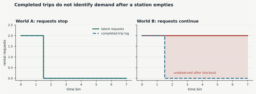
Figure 4:Two worlds can produce the same completed-trip log. In the second world, additional customers attempt to rent while the station is empty. The log cannot identify those censored attempts.
The public station-status feed can report current inventories while it is running, but it does not provide an action channel for relocating bicycles. Historical completed trips omit unsuccessful demand, past station inventories, and operator movements. A fitted arrival model can be useful, but evaluating a new relocation policy from these logs requires assumptions about the missing attempts and about how operations generated the observed data. The executable BIXI example keeps those assumptions visible by declaring an attempted-demand model and recording every rejected event.
Inspect the logged-data counterexample
1 2 3 4 5 6 7 8 9 10 11 12 13 14 15 16 17 18 19 20 21 22 23 24 25 26 27 28 29 30 31 32 33 34 35 36 37 38 39 40 41 42 43 44 45 46 47 48 49 50 51 52 53 54 55 56 57 58 59 60 61 62 63 64 65 66 67def make_censoring_counterexample() -> dict[str, object]: """Two latent request sequences with one identical completed-rental log.""" time = np.arange(8, dtype=int) demand_stops = np.asarray([2, 2, 0, 0, 0, 0, 0, 0], dtype=int) demand_continues = np.asarray([2, 2, 2, 2, 2, 2, 2, 2], dtype=int) def observe(demand: np.ndarray) -> tuple[np.ndarray, np.ndarray]: inventory = 4 completed: list[int] = [] inventories = [inventory] for requested in demand: served = min(int(requested), inventory) completed.append(served) inventory -= served inventories.append(inventory) return np.asarray(completed), np.asarray(inventories) completed_a, inventory_a = observe(demand_stops) completed_b, inventory_b = observe(demand_continues) if not np.array_equal(completed_a, completed_b): raise RuntimeError("the counterexample no longer has identical logs") return { "time": time.tolist(), "demand_stops": demand_stops.tolist(), "demand_continues": demand_continues.tolist(), "completed": completed_a.tolist(), "inventory": inventory_a.tolist(), "logs_identical": bool( np.array_equal(completed_a, completed_b) and np.array_equal(inventory_a, inventory_b) ), } def sha256(path: Path | str) -> str: """Public checksum helper used by artifact builders and tests.""" return _sha256(Path(path)) __all__ = [ "BixiAction", "BixiMetrics", "BixiObservation", "BixiScenario", "BixiTrajectory", "CompletedEventProfile", "Controller", "Event", "EventTrace", "FluidTrajectory", "FrozenScheduleController", "InventoryFeedbackController", "NoRelocationController", "Station", "load_completed_profile", "load_event_trace", "load_scenario", "make_censoring_counterexample", "make_controller", "make_open_loop_controller", "sample_poisson_trace", "sha256", "simulate", "simulate_fluid", ]
Language Generation as a Sequential System
The distinction between a transition model and a policy can also be obscured when one software object appears to generate an entire trajectory. Autoregressive language generation separates the two. For a fixed prompt , let
The base transition appends the selected token,
This transition is deterministic once the token is chosen; uncertainty comes from the token policy . A language model therefore supplies a policy, while the prefix update supplies the transition. A reward or preference model is an additional object rather than an inherent property of text generation.
The simplified boundary changes when the model calls tools, receives new user messages, or interacts with an external application. Tool outputs and user responses then become observations generated by an environment outside the prefix concatenation rule. Context truncation also requires the retained context or memory state to be specified explicitly.
The interface determines which data and counterfactual queries are available. The remaining modeling decision is which transition structure should be fixed and which components should be estimated from those data.
Known Structure and Learned Components
When data expose a mismatch, which model components should be recalibrated and which conservation laws, geometry, and constraints should remain explicit?
Uncertainty in one component does not require replacing the entire model. One can retain the known transition and learn only the discrepancy between its prediction and the observed next state:
The correction is called a learned residual because it accounts for what remains after the known model has made its prediction. The context vector may contain weather, payload information, or other measured conditions. This residual has a narrower task than a complete black-box transition.
| system | retained structure | plausible learned component | model-audit experiment |
|---|---|---|---|
| swing | internal actuation and unilateral tension | rider, damping, and contact-loss parameters | measure the first slack event |
| bicycle corridor | inventory and truck conservation, dock and truck capacities | attempted-demand distribution and travel times | introduce a declared demand shock |
| camera gimbal | rigid-body dynamics, torque limit, and sensor geometry | gyro-bias evolution or disturbance model | separate mechanical rotation from base translation |
| inference service | request, token, and cache conservation | service-rate, power, and thermal residuals | hold out prompt lengths, clocks, and concurrency levels |
| battery cell | charge balance, equivalent circuit, and thermal conservation | resistance change | apply a diagnostic current pulse, then repeat the charge |
Fast Charging When Resistance Drifts
The battery case separates a known model structure from one changed parameter. Charge balance, circuit topology, and thermal conservation remain fixed, while a short current pulse estimates a resistance scale that affects safe charging. This separation makes it possible to ask whether a targeted calibration can correct a specific prediction error without relearning the entire transition.
Charge balance determines how current changes the state of charge. With the book’s charge-positive sign convention,
where is the state of charge, is charging current in amperes, and is cell capacity in ampere-hours. A 5 Ah cell charged at 10 A would move from 20 to 80 percent in
if this were the only relevant equation. Terminal voltage and temperature can restrict the current before that charge target is reached.
Terminal voltage cannot be predicted from charge balance alone because current also produces an immediate resistive rise and a slower polarization response. The reference process represents those two responses with PyBaMM’s documented one-RC Thévenin model Sulzer et al. (2021)Barletta et al. (2022). It also uses two lumped thermal states, treating the cell and its fixture as objects with one uniform temperature each. Its state contains : state of charge, polarization voltage, cell temperature, and jig temperature. The jig is the surrounding fixture with which the cell exchanges heat. The electrical model uses an open-circuit voltage , the cell voltage when no current flows, a series resistance , and an -- branch containing one resistor and one capacitor. Its voltage changes on the time scale , so it represents slower polarization behavior. With denoting terminal voltage, the charge-positive equations are
PyBaMM treats positive current as discharge, so the implementation changes the sign of the positive charging current used in these equations.
The calibration begins with a controlled experiment rather than a full charge. The cell rests at for 20 seconds, receives a commanded 5 A charge current for 10 seconds, and then rests for another 40 seconds. Samples are recorded every 0.5 seconds. Switching the current on produces an immediate voltage jump through , followed by the slower voltage response of the RC branch. Switching it off exposes the decay of that slower response. The pulse is therefore a deliberately chosen input that makes the resistive part of the model visible in the voltage trace.
The committed diagnostic record contains the commanded current, simulated state of charge, and terminal voltage. Independent Gaussian sensor noise with a standard deviation of 1 mV and seed 11 is added to the voltage. This fit does not use temperature measurements. Cell and jig temperatures are monitored in the subsequent full-charge runs, while their model parameters remain fixed.
The nominal circuit uses m, m, and F. The calibration allows only the following one-parameter change:
The dimensionless multiplier measures resistance relative to the nominal circuit. Thus is the nominal cell, and makes both resistances 80 percent larger. The inverse change in keeps the RC time constant at 24 seconds. It is a controlled way to isolate the amplitude of the resistive response, not a claim that all aging changes these three components in this proportion.
Under this restriction, the pulse voltage is linear in . Let denote the polarization voltage predicted at sample by the nominal RC branch, driven by the known current . Define the measured voltage above open circuit and the nominal model’s prediction for that excess voltage as
Thus is the excess voltage observed at sample , while is the excess voltage predicted when the resistance scale is one.
Because the scaled branch has the same time constant and starts from rest, . With denoting voltage-measurement noise, the measured samples therefore satisfy
The estimate chooses the value of that makes the sum of squared voltage prediction errors as small as possible, while restricting the value to a plausible interval:
Before the pulse, both and are zero, so those resting samples contain no information about . The current step makes nonzero, and the relaxation after the step supplies additional samples. This experiment can identify the common multiplier because it is the only unknown in the fit: the ratio and the time constant are fixed. It cannot separately estimate , , and .
The fitted value enters the charging rule as the controller’s resistance estimate . A current governor is a local safety rule that maps the present estimated state to an allowable current request. At each one-second control update, the governor receives the simulated values of , , and and requests the largest current inside three limits. Let and let W/K denote the modeled cell-to-jig heat-transfer coefficient. The rule is
The first entry is the 10 A hardware limit. The second prevents the model’s instantaneous terminal-voltage prediction from exceeding its 4.17 V guard. The third starts from the remaining temperature margin, . Multiplying that margin by gives a simple allowance for resistive heating, modeled here as . Solving this inequality for gives the square-root ceiling in the rule. This ceiling is conservative; it does not forecast the future temperature trajectory. The simulated plant itself is checked against the bounds of 4.20 V and 35 degrees Celsius. A larger fitted resistance lowers both the voltage-based and temperature-based current ceilings.
This governor is a fixed local rule, not an optimization over a future current sequence. Constrained fast charging also motivates richer predictive-control methods Gonzalez-Saenz & Becerra (2024).
The three matched runs ask whether the governor reaches the charge target while respecting its bounds on the reference plant, whether the stale model preserves the voltage margin after resistance changes, and whether updating one parameter restores that margin.
| run | plant scale | governor scale |
|---|---|---|
| fresh, nominal | 1.0 | 1.0 |
| high resistance, stale | 1.8 | 1.0 |
| high resistance, calibrated | 1.8 | fitted from the pulse |
The recorded battery audit compares the three matched runs through charge, terminal voltage, cell temperature, and requested current. Each trace displays only the prefix reached by the playhead. Event controls seek to the first current taper, the first plant-bound violation, and the 80 percent target when those events exist.
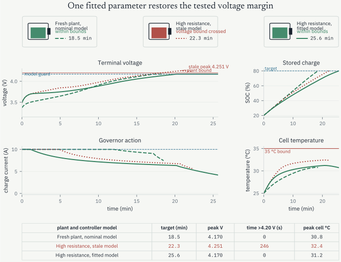
Figure 5:The stale model loses its voltage margin after resistance changes. Updating one fitted resistance scale restores the tested margin at the cost of a longer charge. The online book adds synchronized playback and event seeking.
The pulse-response fit gives alpha = 1.8005. Within the declared one-parameter model, this means that R0 and R1 are estimated to be 1.8005 times their nominal values. The fitted voltage trace has an RMSE of 0.94 mV. The fresh plant reaches the target in 18.52 minutes. The stale model reaches the charge target in 22.26 minutes, but its voltage exceeds 4.20 V for 245.5 seconds and peaks at 4.251 V. The fitted model takes 25.64 minutes and remains inside both plant bounds.
Time above the voltage bound uses linear interpolation at the threshold crossings. The 35 degree C plant bound is never reached, but the conservative 34.5 degree C local thermal-headroom envelope does limit requested current. These are results for a declared teaching cell and a controlled high-resistance counterfactual, not charging guidance for a product.
Within this declared simulation, the comparison supports a narrow conclusion: when the plant differs from the controller model by exactly the common resistance scale above, the pulse estimates that scale well enough for the same governor to remain inside the tested voltage and temperature bounds. The fit changes the predicted voltage drop and resistive heat for a candidate current; it does not replace charge conservation, the circuit topology, or the thermal states.
The comparison does not establish a safe charging rule for a physical product. Every run gives the governor the exact simulated state, so it does not test state estimation. One fitted scale also cannot represent capacity fade, lithium plating, an incorrect open-circuit-voltage curve, sensor bias, spatial temperature gradients, or other electrochemical degradation mechanisms.
Model Predictive Control will optimize an entire future input sequence under state and input constraints. The governor here evaluates a fixed, local current rule so that the consequence of changing one model parameter remains visible.
Inspect the local governor and one-parameter fit
1 2 3 4 5 6 7 8 9 10 11 12 13 14 15 16 17 18 19 20 21 22 23 24 25 26 27 28 29 30 31 32 33 34 35 36 37 38 39 40 41 42 43 44 45 46 47 48 49 50 51 52 53 54 55 56def predictive_current_governor( state: _BatteryState, scenario: BatteryScenario, model_resistance_scale: float, ) -> float: """Return the largest current inside local voltage and thermal envelopes.""" return float( _governed_current( state.soc, state.rc_overpotential_v, state.cell_temperature_c, scenario, model_resistance_scale, maximum=max, minimum=min, square_root=np.sqrt, ) ) def _governed_current( soc: Any, rc_overpotential_v: Any, cell_temperature_c: Any, scenario: BatteryScenario, model_resistance_scale: float, *, maximum: Any, minimum: Any, square_root: Any, ) -> Any: """Evaluate the same local envelope with numeric or PyBaMM operators.""" scaled = resistance_parameters(scenario, model_resistance_scale) voltage_ceiling = maximum( ( scenario.voltage_guard_v - open_circuit_voltage(soc) - rc_overpotential_v ) / scaled["r0_ohm"], 0.0, ) resistance_sum = scaled["r0_ohm"] + scaled["r1_ohm"] thermal_headroom = maximum( scenario.cell_jig_heat_transfer_w_per_k * (scenario.temperature_guard_c - cell_temperature_c), 0.0, ) thermal_ceiling = square_root(thermal_headroom / resistance_sum) return minimum( scenario.current_limit_a, minimum(voltage_ceiling, thermal_ceiling), )
1 2 3 4 5 6 7 8 9 10 11 12 13 14 15 16 17 18 19 20 21 22 23 24 25 26 27 28 29 30 31 32 33 34 35 36 37 38 39 40 41 42 43def fit_resistance_scale( trace: DiagnosticTrace, scenario: BatteryScenario | None = None, ) -> ResistanceFit: """Fit the resistance multiplier by linear least squares on pulse voltage.""" scenario = scenario or BatteryScenario() scenario.validate() if not ( trace.time_s.shape == trace.current_a.shape == trace.soc.shape == trace.measured_voltage_v.shape ): raise ValueError("diagnostic arrays must share one time grid") dt = np.diff(trace.time_s) if np.any(dt <= 0.0): raise ValueError("diagnostic times must increase strictly") base_rc = 0.0 feature = np.empty_like(trace.time_s) tau = scenario.nominal_time_constant_s for index, charge_current in enumerate(trace.current_a): feature[index] = charge_current * scenario.nominal_r0_ohm + base_rc if index + 1 < trace.time_s.size: decay = float(np.exp(-dt[index] / tau)) base_rc = ( decay * base_rc + (1.0 - decay) * charge_current * scenario.nominal_r1_ohm ) centered_voltage = trace.measured_voltage_v - np.asarray( open_circuit_voltage(trace.soc), dtype=float ) informative = np.abs(feature) > 1e-8 if np.count_nonzero(informative) < 2: raise ValueError("diagnostic pulse contains no resistance information") x = feature[informative] y = centered_voltage[informative] unconstrained_scale = float(np.dot(x, y) / np.dot(x, x)) scale = float(np.clip(unconstrained_scale, *RESISTANCE_FIT_BOUNDS)) fitted_voltage = np.asarray(open_circuit_voltage(trace.soc), dtype=float) + scale * feature rmse = float(np.sqrt(np.mean((trace.measured_voltage_v - fitted_voltage) ** 2))) return ResistanceFit(scale, rmse, int(np.count_nonzero(informative)))
Generated simulator or controller code may execute while representing the wrong action, omitting a physical mode, or leaving a safety requirement outside the objective and constraints. Execution tests software behavior. Claims about the target system require inspection of the model and evidence from interventions that expose the disputed assumption.
A residual cannot repair a missing action channel or a missing physical mode if the training data never contains evidence of it. The SwingRL comparison exposed the failure by changing the suspension model while holding the controller fixed. Comparable interventions are needed to decide which structure should remain and which component should be learned.
Exercises
Solution to Exercise 1
One balance consistent with the teaching abstraction is
where and are processed prompt and decode tokens, is the fixed reserve for requests entering decode, is the set that completes, and is all occupancy released by completed request . Equal totals can hide different per-request remaining output lengths, so future completion and cache-release times can differ.
Solution to Exercise 2
The differentiable ODE solver supports chosen-input rollouts and derivatives of those rollouts, which can support shooting or gradient-based MPC. The reset-and-step simulator supports counterfactual sampled rollouts from chosen states and actions, which can support simulation-based MPC, Monte Carlo evaluation, or policy learning. Logged transitions support fitting and evaluation on their recorded distribution, including system identification or fitted Q iteration, but do not by themselves answer arbitrary counterfactual queries.
Solution to Exercise 3
For a closed text prefix, the transition is deterministic concatenation, , while the language model supplies the token distribution . A tool call crosses that boundary. The returned value is an external observation, and the state must retain whatever tool result or interaction history is needed to predict subsequent transitions.
Solution to Exercise 4
The additional customer cannot depart because no bicycle is available. The attempt therefore raises demand by one but generates no completed rental record. Both worlds produce the same observed trip log even though their attempted-demand histories differ.
Solution to Exercise 5
The ten removed prompts each contain 7,436 tokens. For the committed profile, the dilation changes from
The isolated-service total, normalized arrival times, and exogenous request sequence change. The algebraic form of the request, token, cache, and thermal balances does not.
Solution to Exercise 6
The required charge is , so
Because , underestimated resistance makes the governor underpredict terminal voltage and request too much current. Charge conservation, the circuit topology, and the thermal equations remain fixed. During the known 5 A pulse, the immediate voltage jump and slower relaxation make the resistive response visible. Fitting that response estimates the one allowed unknown, , where and are times their nominal values and is divided by . The experiment updates this single controller parameter; it does not relearn the balance equations or separately identify all three circuit elements.
Summary and Outlook
Equations, reset-and-step simulators, logged transitions, and interactive environments expose different operations even when they describe the same nominal evolution. Known balances and constraints can remain explicit while data estimate uncertain parameters, residual dynamics, values, or policies. The battery example makes the division concrete: the circuit and thermal balances remain fixed while one resistance factor is recalibrated.
A model interface can now generate or constrain candidate trajectories. Which admissible action sequence performs best from a given initial condition? The finite-horizon optimal-control problem is the first answer, and it remains open loop until later measurements are allowed to change the decision.
Computational Sources
The SwingRL dependency is pinned to commit
d579663.
The three modeling chapters execute domain code and read committed experiment
artifacts:
The animation controls are embedded in the static site and require no live Python kernel.
- Yu, G.-I., Jeong, J. S., Kim, G.-W., Kim, S., & Chun, B.-G. (2022). Orca: A Distributed Serving System for Transformer-Based Generative Models. 16th USENIX Symposium on Operating Systems Design and Implementation (OSDI 22), 521–538. https://www.usenix.org/conference/osdi22/presentation/yu
- Agrawal, A., Kedia, N., Panwar, A., Mohan, J., Kwatra, N., Gulavani, B. S., Tumanov, A., & Ramjee, R. (2024). Taming Throughput-Latency Tradeoff in LLM Inference with Sarathi-Serve. 18th USENIX Symposium on Operating Systems Design and Implementation (OSDI 24), 117–134. https://www.usenix.org/conference/osdi24/presentation/agrawal
- NVIDIA Corporation. (2026). NVIDIA System Management Interface: nvidia-smi. https://docs.nvidia.com/deploy/nvidia-smi/index.html
- Qwen Team. (2025). Qwen2.5 Technical Report. arXiv Preprint arXiv:2412.15115. https://arxiv.org/abs/2412.15115
- Kwon, W., Li, Z., Zhuang, S., Sheng, Y., Zheng, L., Yu, C. H., Gonzalez, J. E., Zhang, H., & Stoica, I. (2023). Efficient Memory Management for Large Language Model Serving with PagedAttention. Proceedings of the 29th Symposium on Operating Systems Principles, 611–626. 10.1145/3600006.3613165
- Microsoft Azure. (2023). Azure LLM Inference Dataset 2023. Azure Public Dataset. https://github.com/Azure/AzurePublicDataset/blob/master/AzureLLMInferenceDataset2023.md
- Patel, P., Choukse, E., Zhang, C., Shah, A., Goiri, Í., Maleki, S., & Bianchini, R. (2024). Splitwise: Efficient Generative LLM Inference Using Phase Splitting. Proceedings of the 51st Annual International Symposium on Computer Architecture (ISCA). https://www.microsoft.com/en-us/research/publication/splitwise-efficient-generative-llm-inference-using-phase-splitting/
- Qwen Team. (2025). Qwen2.5-7B-Instruct, revision acbd96531cda22292a3ceaa67e984955d3965282. Hugging Face model repository. https://huggingface.co/Qwen/Qwen2.5-7B-Instruct/tree/acbd96531cda22292a3ceaa67e984955d3965282
- vLLM Project. (2026). Using Docker with vLLM, version 0.28.0. https://docs.vllm.ai/en/v0.28.0/deployment/docker/
- Sulzer, V., Marquis, S. G., Timms, R., Robinson, M., & Chapman, S. J. (2021). Python Battery Mathematical Modelling (PyBaMM). Journal of Open Research Software, 9(1), 14. 10.5334/jors.309
- Barletta, G., Di Prima, P., & Papurello, D. (2022). Thévenin’s Battery Model Parameter Estimation Based on Simulink. Energies, 15(17), 6207. 10.3390/en15176207
- Gonzalez-Saenz, J., & Becerra, V. (2024). Determining Fast Battery Charging Profiles Using an Equivalent Circuit Model and a Direct Optimal Control Approach. Energies, 17(6), 1470. 10.3390/en17061470