Controlled Systems: Boundaries, States, and Actions - Building Up RL: From Dynamics and Control to Learning

The introduction identified the state, action, evolution, objective, and constraints as the ingredients of a sequential decision problem. Before any algorithm can compare actions, how can those ingredients be tied to one physical system and one decision maker?

A simulated playground swing can be made easy to control by placing a motor at the suspension pivot. A rider on a real swing has no such motor. The rider can change body shape, and the chain can pull but cannot push. An optimizer may produce a successful trajectory for the first model even though neither its action nor its suspension exists in the target system.

This failure occurs before the choice of control or learning algorithm. A decision model must say what evolves, what can be observed, which interventions are possible, how uncertainty enters, and which constraints must hold. Its information pattern specifies what the decision maker knows when each action is selected. These choices lead from physical systems to state-space equations and then to simulators, logged transitions, and interactive environments. Each case study tests one part of the resulting model.

Trajectory optimization, model predictive control, dynamic programming, and reinforcement learning all reason about the consequences of actions. They can only compare consequences that the model makes possible, including the predicted outcome of an action that has not yet been tried. Such an unobserved alternative is called a counterfactual. A fictitious actuator creates infeasible plans, an incomplete state destroys predictive information, and a logged dataset cannot answer counterfactual questions about actions it does not cover. Modeling therefore determines which later computations and claims are meaningful.

The modeling choices have a useful dependency order. The system boundary first separates internal variables from external influences. That boundary determines the state, observation, action, and disturbance. Dynamics then describe how these quantities interact, while the objective and constraints define the decision problem. Finally, the available model interface determines whether an algorithm can differentiate equations, run new simulations, or only analyze a fixed log. The chapter follows this order.

System Boundaries and Action Channels¶

Which physical variables belong inside the controlled system, and which interventions can the decision maker actually apply across that boundary?

A playground swing, an overhead crane, and a wave-energy converter all oscillate. Their visual similarity does not make them the same control problem. A rider changes body shape, a crane accelerates the suspension point, and a wave-energy converter changes a dissipative load while the sea supplies the forcing.

The boundary identifies which physical components belong to the system being modeled and which influences arrive from outside it. The action channel then identifies the intervention available to the decision maker within that boundary. These two choices must precede the equations because they determine which input terms the equations are allowed to contain.

from pathlib import Path
import sys

import matplotlib.pyplot as plt
import numpy as np
from IPython.display import HTML, display

code_dir = Path.cwd() / "code"
if str(code_dir) not in sys.path:
    sys.path.insert(0, str(code_dir))

from modeling_interfaces import make_overview_figure

<Figure size 1230x465 with 3 Axes> — Figure 1:The systems share an oscillatory silhouette but expose different control interfaces. The rider changes internal shape, the crane accelerates its pivot, and the wave device changes a nonnegative dissipative load. Their desired motions and feasible actions therefore differ.

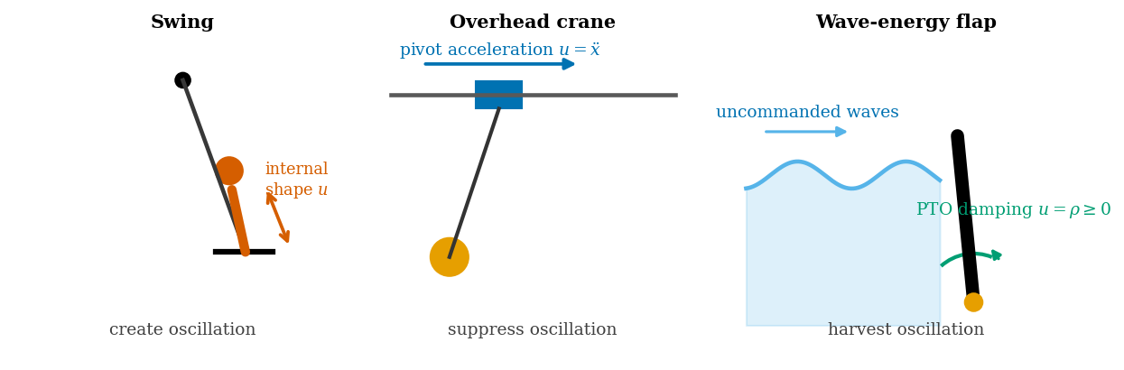
system	state must describe	action changes	external influence	objective	hard constraint
playground swing	suspension angle and rider pose	internal body shape	gravity and drag	add mechanical energy	a chain can pull but cannot push
overhead crane	trolley position and load angle	trolley acceleration	gravity and damping	move the load and remove sway	acceleration is bounded
wave-energy converter	flap angle and velocity	power-take-off damping	incident waves	extract energy within motion limits	passive damping is nonnegative

Solution to Exercise 1

The rider creates oscillation by changing body shape. The crane suppresses load sway by changing trolley acceleration. The wave-energy converter retains motion while extracting energy by changing nonnegative power-take-off damping. The systems look similar, but none exposes an arbitrary force at the oscillating coordinate.

The three systems need different inputs, but their mechanical equations can be organized by the same bookkeeping template. Let $q$ collect the independent coordinates needed to describe configuration, such as an angle or a trolley position. Such coordinates are called generalized positions. Their velocities are $v=\dot q$ ; $z$ collects additional actuator or environment states; and $u$ is the commanded input. A broad finite-dimensional model is

\dot q=v, \qquad M(q,z)\dot v+c(q,v,z,\dot z)+\nabla_q V(q,z)+r(q,v,z) =B(q,v,z)u+G(q,v,z)\xi_v(t), \qquad \dot z=g(q,v,z,u,\xi_z(t)).

(1)

The mass matrix $M$ maps coordinate accelerations to their corresponding forces or torques, collectively called generalized forces. It is positive definite, which ensures that every nonzero velocity has positive kinetic energy. The term $c$ collects velocity- and configuration-dependent inertial forces, including Coriolis and centrifugal effects. The gradient $\nabla_q V$ appears on the left side, so the corresponding conservative force is $-\nabla_q V$ . The term $r$ represents dissipative resistance. The columns of $B$ and $G$ specify the physical directions through which actions $u$ and external inputs $\xi=(\xi_v,\xi_z)$ enter. Dissipation requires $v^\top r(q,v,z)\geq0$ , so resistance cannot add mechanical energy. An action can enter directly through $Bu$ or indirectly by changing $z$ . A moving coordinate whose inertia is modeled belongs in $q$ ; a fixed parameter or prescribed signal does not need its own state equation.

The term $B(q,v,z)u$ cannot be inferred from the word “action” alone. An unconstrained vector input would omit the swing’s internal-actuation geometry, the crane’s acceleration limit, and the wave device’s passivity restriction.

Optional connection: port-Hamiltonian models

The mechanical template above is one coordinate-level instance of a broader energy-based description. A port-Hamiltonian model writes

\dot x=[J(x)-R(x)]\nabla H(x)+G(x)u, \qquad y=G(x)^\top\nabla H(x),

(2)

where $H$ stores energy, the skew-symmetric matrix $J$ routes energy, $R$ dissipates it, and $(u,y)$ form an external power port. The same structure can connect mechanical, electrical, fluid, and thermal components. When $H$ has no explicit time dependence, its energy balance is

\dot H=-\nabla H(x)^\top R(x)\nabla H(x)+y^\top u.

(3)

The first term dissipates stored energy, while $y^\top u$ is power supplied through the port Schaft & Jeltsema (2014). This chapter uses the more concrete coordinate form.

The system boundary also determines which variables are external. At sea, the incident wave torque is an uncommanded disturbance to the energy converter. In a laboratory wave tank, an experimenter can command a motorized paddle that generates the waves. The paddle command is then an action, while the resulting hydrodynamic torque remains a force on the flap. The converter has not changed; the modeled boundary, decision maker, and physical actuator have.

Once the boundary and action channel are fixed, the remaining internal variables must be summarized in a form that predicts what happens next. That predictive summary is the state.

State-Space Models¶

Once the boundary and action channel are fixed, which variables summarize the past well enough to predict the effect of the next action?

A state summarizes the past information needed to predict future evolution under a chosen action. The word “needed” depends on the model. For example, indoor air temperature alone may fail to predict the next temperature if heat stored in the walls is omitted. Two rooms with the same air temperature but different wall temperatures respond differently after the heater is turned off. Adding wall temperature to the state removes that ambiguity in a simple thermal model.

Once the state has been chosen, it should make earlier history unnecessary for one-step prediction. For a stochastic discrete-time model, this requirement is the Markov property:

\Pr(x_{t+1}\in A\mid x_{0:t},u_{0:t}) =\Pr(x_{t+1}\in A\mid x_t,u_t),

(4)

for every set $A$ of possible next states. The left side conditions on the entire state-action history, while the right side retains only the current state and action. Their equality means that the older history supplies no additional information about the next state. The definition is relative to the declared model and time scale. A simulator may store a large internal state while exposing a smaller observation to the controller, and that observation need not itself be Markov.

A state-space model can keep disturbances and sensor errors as explicit inputs. In discrete time, such a model has the form

x_{t+1}=f_t(x_t,u_t,\xi_t), \qquad y_t=h_t(x_t,u_t,\nu_t).

(5)

Here $f_t$ advances the state, while $h_t$ maps the state and action to the sensor output $y_t$ . The variable $\xi_t$ is a process disturbance that changes the physical evolution, whereas $\nu_t$ is measurement noise that changes only the reported observation. For fixed values of these inputs, both equations are deterministic maps. The stochastic section later assigns probability laws to them.

In continuous time, the corresponding equations are

\dot x(t)=f(x(t),u(t),\xi(t)), \qquad y(t)=h(x(t),u(t),\nu(t)).

(6)

The first equation specifies a rate of change rather than a one-step update. Many physical laws are most compact in continuous time because mechanics, circuit theory, fluid dynamics, heat transfer, and chemical kinetics describe rates, flows, and conservation balances. Those fields provide reusable structure: geometry, conservation laws, units, and admissible energy flows need not be relearned from trajectories. Unknown parameters or empirical relationships, such as drag or heat-transfer laws, can instead be estimated inside that structure.

Continuous equations still need a sampling convention before a digital controller can use them. Sensors and command interfaces operate at discrete times even though the physical plant continues to evolve between updates. Under a chosen hold rule, which specifies how an action is maintained between updates, and a sampling period $\Delta t$ , integrating the ODE defines a discrete transition $x_{k+1}=F_{\Delta t}(x_k,u_k)$ . The map $F_{\Delta t}$ is called the exact flow over one sample interval. A numerical integrator approximates this map. Changing $\Delta t$ or the hold changes the sampled transition, not the underlying physical law. It can also change the disturbance model because a short event may be visible on one sampling grid and absent from another.

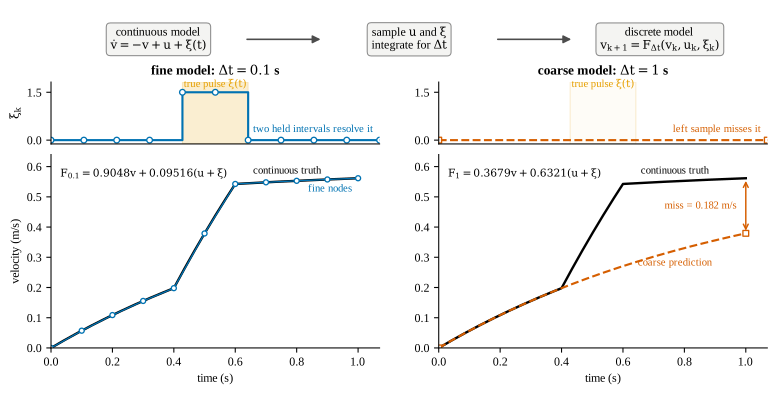
A continuous scalar velocity model is sampled at fine and coarse periods. The fine zero-order-hold disturbance representation captures a short pulse, while the coarse left-endpoint representation misses it and predicts the wrong endpoint. — Figure 2:A sampling period and an interval integrator jointly define the discrete transition. The action is held at $0.6\ \mathrm{m/s^2}$ , and the true disturbance acts only from 0.4 to 0.6 seconds. At $\Delta t=0.1$ seconds, its two sampled intervals reproduce the $0.182\ \mathrm{m/s}$ endpoint contribution. At $\Delta t=1$ second, the left-endpoint disturbance sample is zero, so the held coarse model predicts $0.379\ \mathrm{m/s}$ instead of $0.562\ \mathrm{m/s}$ . The ODE and interval integrator are unchanged; the sampling period changes both $F_{\Delta t}$ and what the sampled disturbance representation can express.

Coarse output sampling alone does not erase a known event. An integrator given the true event time and $\xi(t)$ can still resolve the pulse with internal substeps. The miss in Figure 2 occurs because the coarse model replaces $\xi(t)$ by left-endpoint, zero-order-held samples. Here zero-order hold means that each sampled value is kept constant until the next sample.

The general nonlinear maps above can be difficult to analyze or optimize. Linear state-space models provide a tractable local or exact special case:

\dot x=Ax+Bu+E\xi, \qquad y=Cx+Du.

(7)

The matrix $A$ describes autonomous state evolution, $B$ describes how the action changes that evolution, and $E$ describes how disturbances enter. The matrix $C$ selects or combines state components into measurements, while $D$ captures any immediate effect of the action on the measurement. Thus $B$ and $C$ encode different questions. An actuator may be able to influence every state direction without sensors measuring every state component. Conversely, measuring the full state does not imply that the available actuators can move it in every direction.

Linearity is a modeling choice rather than a claim that the world is linear at all scales. A nonlinear system may be well approximated by a linear model near an equilibrium. Dynamic programming itself is not restricted to linear models or stabilization: its Bellman recursion also applies to nonlinear and stochastic transitions. In the later inverted-pendulum example, a local linear approximation supplies one stabilizing controller, while Trajectory Optimization uses the nonlinear equations to move the pendulum into that controller’s local region.

Dynamics answer the counterfactual question “what happens after this action?” A decision problem must additionally specify which consequences are preferred, which are forbidden, and what information may be used when each action is chosen.

Decision Problems and Policy Classes¶

A state-space model predicts evolution under an input, but which objective, constraints, and information pattern turn that prediction into a decision problem?

In machine learning, a model often means a parameterized predictor. A decision model contains more: a state, available actions, dynamics, observations, an objective, constraints, and an information pattern. Prediction remains one component, but decisions require counterfactual trajectories under actions that may not yet have been observed.

For a finite horizon of $T$ actions, let $P_t(\cdot\mid x,u)$ be the distribution of the next state after applying action $u$ in state $x$ . The set $\mathcal U_t(x)$ contains the feasible actions, and $\mathcal X_t$ contains the admissible states. A stage cost $\ell_t(x,u)$ evaluates one decision, while $\ell_T(x)$ evaluates the terminal state. A feedback policy $\pi_t$ maps the available information $I_t$ to an action. These objects define the problem

\begin{aligned} \underset{\pi_0,\ldots,\pi_{T-1}}{\operatorname{minimize}}\quad & \mathbb{E}^{\pi}\!\left[\sum_{t=0}^{T-1} \ell_t(x_t,u_t)+\ell_T(x_T)\right] \\ \text{subject to}\quad & x_{t+1}\sim P_t(\cdot\mid x_t,u_t), \\ & u_t=\pi_t(I_t)\in\mathcal U_t(x_t), \\ & x_t\in\mathcal X_t \quad \text{almost surely}. \end{aligned}

(8)

The expectation averages the accumulated cost over trajectories generated by the policy and stochastic dynamics. The state constraint holds almost surely, meaning with probability one under that trajectory distribution. Replacing it by a constraint on the average value, or by a chance constraint that permits a stated probability of violation, would define a different feasible set. Thus the formulation specifies what is optimized, how uncertainty propagates, which information a policy may use, and which trajectories are admissible. Omitting one of these pieces changes the problem even if the same environment class and neural network are used afterward.

An open-loop plan selects the whole action sequence from information available at the start,

(u_0,\ldots,u_{T-1})=\mu(I_0).

(9)

The sequence remains fixed after planning. A feedback policy instead selects each action from the information available at that time,

u_t=\pi_t(I_t).

(10)

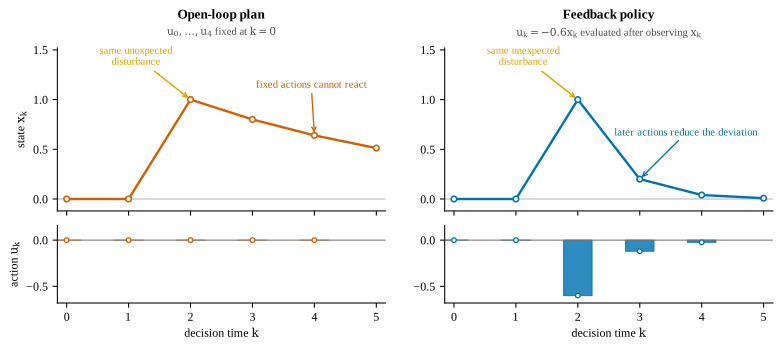
Two controllers face the same unexpected disturbance. The open-loop controller keeps its precomputed actions, while the feedback controller changes later actions after observing the displaced state. — Figure 3:An open-loop plan commits to future actions before the trajectory begins. A feedback policy reevaluates its decision rule after each new observation. The rule may be an optimizer, a learned policy, or a hand-written heuristic; the word *feedback* describes what information reaches the action, not how the rule was obtained. In this illustration, $x_{k+1}=0.8x_k+u_k+\xi_k$ : the open-loop schedule contains zeros, while the feedback rule $u_k=-0.6x_k$ responds after the disturbance becomes visible at $x_2$ . The example shows information flow, not a guarantee that every feedback rule performs well.

A planned trajectory can perform well under its assumed initial condition and disturbance forecast while reacting poorly to a tap, a delayed actuator, or an unexpected arrival. Later chapters construct open-loop plans, turn them into feedback by replanning, and compute state-contingent value functions.

The policy class and the model are separate choices. Several independent axes describe the model itself.

axis	common alternatives	consequence
time	continuous or discrete	differential equations or transition steps
evolution	deterministic or stochastic	one next state or a distribution over next states
state	continuous, discrete, or mixed	geometry of the state space and applicable solvers
action	continuous, discrete, or mixed	control authority and optimization method
observation	full state or partial/noisy measurement	state feedback or estimation from information histories
horizon	finite, infinite, or terminating	terminal conditions and objective definition

Terms such as “continuous control” specify only one row of this table. They do not determine the time representation, uncertainty, observation model, or information available to the controller.

The swing example now combines these modeling choices. Its action is continuous, its plant is simulated in continuous time, its feedback rule uses observations at discrete times, and its suspension constraint changes the equations when the chain becomes slack. The comparison isolates what goes wrong when the action channel or constraint is modeled incorrectly.

Internal Actuation and Unilateral Constraints in SwingRL¶

How can a concrete model audit reveal that a nominally successful controller relies on an actuator or contact force the real system cannot produce?

A rider who wants to swing higher cannot command a torque at the suspension pivot. The available interventions are changes in body shape, and the chain can transmit tension but not compression. A complete revolution provides a strict test of both assumptions: the controller must inject enough energy through internal motion while remaining feasible for a unilateral suspension.

The swing-rl environment turns those requirements into a control problem. Its articulated standing model exposes two normalized actions in $[-1,1]^2$ : a squat target and a torso-lean target. The action changes body geometry rather than applying a hidden torque at the suspension pivot.

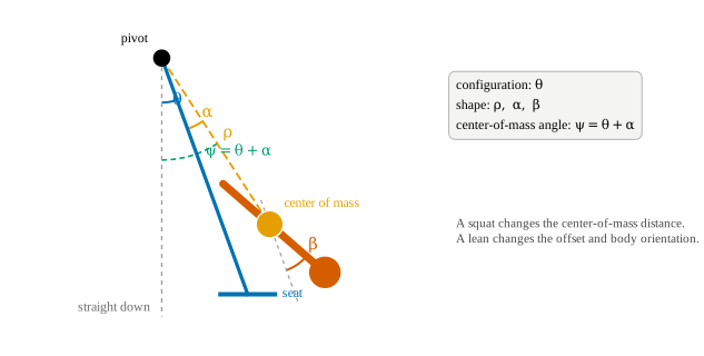
Geometry of the reduced swing model, showing the suspension angle theta, pivot-to-center-of-mass distance rho, center-of-mass offset alpha, absolute center-of-mass angle psi, and body angle beta. — Figure 4:The reduced coordinates describe the rider in aggregate rather than tracking every joint. The suspension angle is $\theta$ . The center of mass lies a distance $\rho$ from the pivot and is offset by $\alpha$ from the suspension, so its absolute angle is $\psi=\theta+\alpha$ . The angle $\beta$ describes the body’s orientation relative to the suspension. Squatting mainly changes $\rho$ ; leaning changes $\alpha$ and $\beta$ .

The reduced model makes the internal action channel visible in one equation. Let $m$ be the rider’s mass, $g$ gravitational acceleration, $\theta$ the suspension angle, $\rho$ the center-of-mass distance from the pivot, $\alpha$ its offset from the suspension line, $\psi=\theta+\alpha$ , $\beta$ the body orientation relative to the suspension, and $J$ the rider’s inertia about its center of mass. With $\tau_{\mathrm{damp}}$ denoting the modeled damping torque, the suspension-coordinate balance is

(m\rho^2+J)\ddot\theta =-m\rho^2\ddot\alpha -2m\rho\dot\rho\dot\psi -J\ddot\beta -\dot J(\dot\theta+\dot\beta) -mg\rho\sin\psi +\tau_{\mathrm{damp}}.

(11)

There is no commanded pivot torque on the right side. Torso lean instead contributes through the acceleration terms in $\ddot\alpha$ and $\ddot\beta$ , while squatting changes $\rho$ and contributes through $-2m\rho\dot\rho\dot\psi$ . Multiplying this generalized force by the angular velocity $\dot\theta$ gives its mechanical power. Near a bottom passage, $\dot\psi\approx\dot\theta$ , so the squat contribution is approximately

\left(-2m\rho\dot\rho\dot\psi\right)\dot\theta \approx -2m\rho\dot\rho\dot\theta^2.

(12)

Shortening means $\dot\rho<0$ . Since $m>0$ , $\rho>0$ , and $\dot\theta^2\geq0$ , the contribution is positive in either direction of travel. The model therefore explains how a rider can add energy without a fictitious pivot actuator.

The action channel is only half of the audit; the suspension must also obey the correct force constraint. The matched comparison applies one phase-feedback law, a rule that times squat and lean targets from the observed oscillation phase, to the standing body under two suspension models supplied by SwingRL. A rigid rod can carry tension or compression. A chain can pull but cannot push. The body parameters, initial state, squat and lean limits, feedback rule, 32-second horizon, and 0.02-second sampling interval remain fixed. During the first 0.25 seconds, both runs multiply their requested squat and lean targets by

r(t)=\min(t/0.25,1)

(13)

so both commands rise linearly from zero to their full requested values instead of jumping at the first step. This shared startup ramp prevents an initial command discontinuity from being counted as a chain-release event.

Success requires the unwrapped suspension angle to change by at least $2\pi$ , one complete revolution. At that crossing, the pivot-to-seat distance must also be at least $0.9L$ , where $L$ is the fully extended suspension length. The second test prevents a rotation from being credited while the seat is bunched close to the pivot.

Both simulations use the same function from the current observation to squat and lean commands. Once the chain releases, however, the rod and chain follow different trajectories and produce different observations. Applying the same feedback function to those different observations can produce different later commands. The comparison therefore holds the feedback rule fixed, not the entire open-loop command sequence.

The recorded comparison below applies that feedback rule to both suspension models. The left plant permits axial force in either direction, while the right plant enforces a chain that can only pull. Each plot displays the trajectory only up to the selected playback time. The unwrapped angle keeps accumulating past $\pm\pi$ , so a full revolution remains visible. The compression-demand trace shows how much pushing force the rod trajectory would require, a force the chain cannot supply. The extension trace shows the pivot-to-seat distance relative to $L$ . Event buttons jump to times already located in the Python trajectory: chain release, impact on reattachment (the snap), and the rod run’s first completed revolution.

from pathlib import Path
import sys

from IPython.display import HTML, display

code_dir = Path.cwd() / "code"
if str(code_dir) not in sys.path:
    sys.path.insert(0, str(code_dir))

from swing_control import model_audit_player_html

display(HTML(model_audit_player_html(
    Path("_static/swing_modeling"),
    Path("artifacts/swing_modeling/events.json"),
    fallback_id="fig-swing-model-audit-fallback",
)))

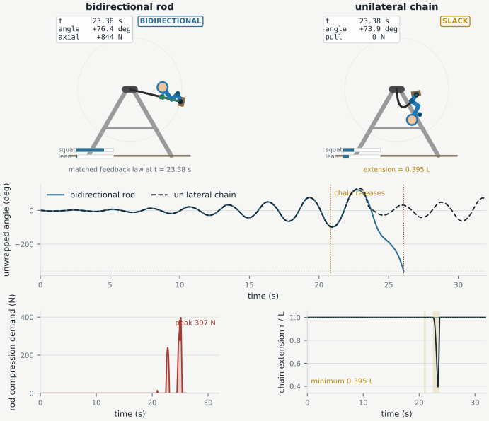
Matched SwingRL rod and chain keyframes with complete traces for angle, rod compression demand, and chain extension. — Figure 5:Matched keyframes and complete diagnostics from the same Python trajectories. The online book adds the recorded 16:9 animation and event seeking.

Suspension model	Full rotation	Peak $\lvert\theta\rvert$	Minimum axial force	Minimum $r/L$	Slack time
Bidirectional rigid rod	yes, 26.08 s	361.16°	-397.1 N	1.000	0.00 s
Unilateral chain	no	130.49°	0.0 N	0.395	1.61 s

The rod trajectory requests as much as 397.1 N of compression, which a chain cannot provide. The chain first releases at 20.84 s, releases 2 times in total, and loses 1380.6 J across reattachments.

Recorded chain mode changes:

Release at 20.84 s ( $\theta=-97.2^\circ$ ).
Reattachment at 21.22 s ( $\theta=-90.6^\circ$ ).
Release at 22.46 s ( $\theta=114.9^\circ$ ).
Reattachment at 23.68 s ( $\theta=10.9^\circ$ ).

The rod completes a rotation, but part of that motion requires the suspension to push the seat away from the pivot. A real chain cannot supply that push. It goes slack when the pulling force would otherwise become negative, and the seat and rider then move freely under gravity until the chain becomes fully extended again. At that instant the chain snaps taut, the velocity changes abruptly, and some mechanical energy is lost. In modeling language, this is a hybrid system: it switches between taut and slack equations and includes a reset at reattachment. Changing a coefficient in the always-taut rod equation cannot create the missing free-flight mode or the snap.

This controller completes the task on the bidirectional-rod model and fails on the unilateral-chain plant. The comparison does not rank control against reinforcement learning, nor does it establish that a chain swing cannot be rotated. It isolates a physical assumption: success on the rod model provides no evidence that the same trajectory remains feasible when the suspension cannot push.

A learned approximation fitted only to rod trajectories would inherit the same blind spot. Data remain useful for estimating rider parameters, damping, and contact losses after the unilateral mode structure is represented. Policy Gradients later evaluates PPO and the structured controller against the same SwingRL action semantics and success criterion.

The swing audit changed a structural constraint while keeping the decision rule fixed. The next modeling question concerns outcomes that vary even when the state and action are fixed, such as demand arrivals or environmental disturbances.

swing_control.py

1
2
3
4
5
6
7
8
9
10
11
12
13
14
15
16
17
18
19
20
21
22
23
24
25
26
27
28
29
30
31
32
33
34
35
36
37
38
39
40
41
42
43
44
45
46
47
48
49
50
51
52
53
54
55
56
57
58
59
60
61
62
63
64
65
66
67
68
69
70
71
72
73
74
75
76
77
78
79
80
81
82
83
84
85
86
87
88
89
90
91
92
93
94
95
96
97
98
99
100
101
102
103
104
105
106
107
108
109
110
111
112
113
114
115
116
117
118
119
120
121
122
123
124
125
126
127
128
129
130
131
132
133
134
135
136
137
138
139
140
141
142
143
144
145
146
147
148
149
150
151
152
153
154
155
156
157
158
159
160
161
162
163
164
165
166
167
168
169
170
171
172
173
174
175
176
177
178
179
180
181
182
183
184
185
186
187
188
189
190
191
192
193
194
195
196
197
198
199
200
201
202
203
204
205
206
207
208
209
210
211
212
213
214
215
216
217
218
219
220
221
222
223
224
225
226
227
228
229
230
231
232
233
234
235
236
237
238
239
240
241
242
243
244
245
246
247
248
249
250
251
252
253
254
255
256
257
258
259
260
261
262
263
264
265
266
267
268
269
270
271
272
273
274
275
276
277
278
279
280
281
282
283
284
285
286
287
288
289
290
291
292
293
294
295
296
297
298
299
300
301
302
303
304
305
306
307
308
309
310
311
312
313
314
315
316
317
318
319
320
321
322
323
324
325
326
327
328
329
330
331
332
333
334
335
336
337
338
339
340
341
342
343
344
345
346
347
348
349
350
351
352
353
354
355
356
357
358
359
360
361
362
363
364
365
366
367
368
369
370
371
372
373
374
375
376
377
378
379
380
381
382
383
384
385
386
387
388
389
390
391
392
393
394
395
396
397
398
399
400
401
402
403
404
405
406
407
408
409
410
411
412
413
414
415
416
417
418
419
420
421
422
423
424
425
426
427
428
429
430
431
432
433
434
435
436
437
438
439
440
441
442
443
444
445
446
447
448
449
450
451
452
453
454
455
456
457
458
459
460
461
462
463
464
465
466
467
468
469
470
471
472
473
474
475
476
477
478
479
480
481
482
483
484
485
486
487
488
489
490
491
492
493
494
495
496
497
498
499
500
501
502
503
504
505
506
507
508
509
510
511
512
513
514
515
516
517
518
519
520
521
522
523
524
525
526
527
528
529
530
531
532
533
534
535
536
537
538
539
540
541
542
543
544
545
546
547
548
549
550
551
552
553
554
555
556
557
558
559
560
561
562
563
564
565
566
567
568
569
570
571
572
573
574
575
576
577
578
579
580
581
582
583
584
585
586
587
588
589
590
591
592
593
594
595
596
597
598
599
600
601
602
603
604
605
606
607
608
609
610
611
612
613
614
615
616
617
618
619
620
621
622
623
624
625
626
627
628
629
630
631
632
633
634
635
636
637
638
639
640
641
642
643
644
645
646
647
648
649
650
651
652
653
654
655
656
657
658
659
660
661
662
663
664
665
666
667
668
669
670
671
672
673
674
675
676
677
678
679
680
681
682
683
684
685
686
687
688
689
690
691
692
693
694
695
696
697
698
699
700
701
702
703
704
705
706
707
708
709
710
711
712
713
714
715
716
717
718
719
720
721
722
723
724
725
726
727
728
729
730
731
732
733
734
735
736
737
738
class SwingScenario:
    """The matched model-audit scenario used in the modeling chapter."""

    horizon_seconds: float = 32.0
    control_interval: float = 0.02
    integrator_substeps: int = 8
    success_angle: float = 2.0 * math.pi
    success_radius_fraction: float = 0.9
    initial_angle: float = 0.0
    initial_angular_velocity: float = 0.0
    seed: int = 0
    command_ramp_seconds: float = 0.25

    @property
    def maximum_steps(self) -> int:
        return int(round(self.horizon_seconds / self.control_interval))


DEFAULT_SWING_SCENARIO = SwingScenario()

_STANDING_PRESET = ArticulatedPumper.standing(1.0)
STANDING_PUMP_CHANNELS = tuple(_STANDING_PRESET.channels)
STANDING_STARTUP_AMPLITUDE = float(_STANDING_PRESET.startup_amplitude)


def structured_standing_actions(
    observations: Any,
    time_step: Any,
    natural_frequency: float,
    scenario: SwingScenario = DEFAULT_SWING_SCENARIO,
    *,
    array_module: Any = np,
) -> Any:
    """Evaluate SwingRL's standing phase law with the shared startup ramp.

    ``array_module`` may be NumPy or ``jax.numpy``.  The channel harmonics,
    phases, and startup threshold come directly from SwingRL's
    :meth:`ArticulatedPumper.standing` preset.  This functional form lets PPO
    evaluate the same controller over a batch without maintaining Python
    controller objects inside a JAX scan.
    """

    xp = array_module
    values = xp.asarray(observations)
    psi = xp.arctan2(values[..., 4], values[..., 3])
    psi_dot = values[..., 5] * natural_frequency
    cosine_amplitude = xp.cos(psi) - xp.square(psi_dot) / (
        2.0 * natural_frequency**2
    )
    amplitude = xp.arccos(xp.clip(cosine_amplitude, -1.0, 1.0))
    phase = xp.arctan2(-psi_dot / natural_frequency, psi)
    elapsed = (time_step + 1) * scenario.control_interval
    clock = natural_frequency * elapsed
    source = xp.where(amplitude < STANDING_STARTUP_AMPLITUDE, clock, phase)
    actions = xp.stack(
        [
            gain * xp.sin(harmonic * source + phase_offset)
            for harmonic, phase_offset, gain in STANDING_PUMP_CHANNELS
        ],
        axis=-1,
    )
    if scenario.command_ramp_seconds > 0.0:
        envelope = xp.minimum(elapsed / scenario.command_ramp_seconds, 1.0)
        actions = actions * envelope
    return xp.clip(actions, -1.0, 1.0)


@dataclass
class RampedStandingController:
    """SwingRL's standing pumper with a short ramp from the neutral pose.

    The phase law remains SwingRL's :class:`ArticulatedPumper`.  The common
    ramp prevents an instantaneous initial target change from becoming the
    first chain-release event in the teaching comparison.
    """

    natural_frequency: float
    control_interval: float = 0.02
    ramp_seconds: float = 0.25
    _controller: ArticulatedPumper = field(init=False, repr=False)
    _elapsed: float = field(init=False, default=0.0, repr=False)

    def __post_init__(self) -> None:
        self._controller = ArticulatedPumper.standing(
            self.natural_frequency,
            dt=self.control_interval,
        )

    def reset(self) -> None:
        self._controller.reset()
        self._elapsed = 0.0

    def __call__(self, observation: np.ndarray) -> np.ndarray:
        action = np.asarray(self._controller(observation), dtype=np.float32)
        self._elapsed += self.control_interval
        if self.ramp_seconds <= 0.0:
            return action
        scale = min(self._elapsed / self.ramp_seconds, 1.0)
        return np.asarray(scale * action, dtype=np.float32)


@dataclass(frozen=True)
class SwingTrace:
    """A SwingRL rollout with the diagnostics needed for a model audit."""

    name: str
    rollout: Rollout
    target_actions: np.ndarray
    realized_commands: np.ndarray
    seat_radius: np.ndarray
    taut: np.ndarray
    slack_time: np.ndarray
    snap_energy_loss: np.ndarray

    @property
    def times(self) -> np.ndarray:
        return self.rollout.times

    @property
    def angles(self) -> np.ndarray:
        return self.rollout.thetas

    @property
    def energies(self) -> np.ndarray:
        return self.rollout.energies

    @property
    def tensions(self) -> np.ndarray:
        return self.rollout.tensions


def make_environment(
    scenario: SwingScenario = DEFAULT_SWING_SCENARIO,
    *,
    suspension: str,
    reset_noise: float = 0.0,
) -> tuple[SwingParams, SwingEnv]:
    """Construct a matched rigid-rod or unilateral-chain SwingRL plant."""

    parameters = SwingParams()
    integrator = IntegratorParams(
        dt=scenario.control_interval,
        substeps=scenario.integrator_substeps,
    )
    reward = RewardParams(
        success_angle=scenario.success_angle,
        success_radius_fraction=scenario.success_radius_fraction,
    )
    common = {
        "swing": parameters,
        "integrator": integrator,
        "reward": reward,
        "max_episode_steps": scenario.maximum_steps,
        "reset_noise": reset_noise,
    }
    if suspension == "rigid_rod":
        model = articulated_standing(parameters)
        environment = SwingEnv(
            model=model,
            rider=rider_for(model, parameters),
            **common,
        )
    elif suspension == "unilateral_chain":
        environment = make_chain_env(
            body="articulated_standing",
            **common,
        )
    else:
        raise ValueError(
            "suspension must be 'rigid_rod' or 'unilateral_chain'"
        )
    return parameters, environment


def make_structured_controller(
    parameters: SwingParams,
    scenario: SwingScenario = DEFAULT_SWING_SCENARIO,
) -> RampedStandingController:
    """Return the shared feedback controller for the model audit."""

    return RampedStandingController(
        natural_frequency=parameters.natural_frequency,
        control_interval=scenario.control_interval,
        ramp_seconds=scenario.command_ramp_seconds,
    )


def _hybrid_diagnostics(environment: SwingEnv) -> tuple[bool, float, float]:
    rendered = environment.render_state()
    taut = bool(rendered.get("taut", True))
    state = environment._state
    slack = float(getattr(state, "slack_time", 0.0))
    loss = float(getattr(state, "energy_lost", 0.0))
    return taut, slack, loss


def simulate_controller(
    environment: SwingEnv,
    controller: Callable[[np.ndarray], np.ndarray],
    scenario: SwingScenario = DEFAULT_SWING_SCENARIO,
    *,
    name: str,
) -> SwingTrace:
    """Run one deterministic closed-loop episode and retain audit diagnostics."""

    observation, _ = environment.reset(
        seed=scenario.seed,
        options={
            "theta": scenario.initial_angle,
            "theta_dot": scenario.initial_angular_velocity,
            "noise": 0.0,
        },
    )
    if hasattr(controller, "reset"):
        controller.reset()

    rollout = Rollout(length=environment.model.nominal_length)
    rollout.append(environment)
    zero_action = np.zeros(environment.action_space.shape, dtype=np.float32)
    target_actions = [zero_action]
    realized_commands = [rollout.frames[-1].commands.copy()]
    seat_radius = [float(np.linalg.norm(rollout.frames[-1].seat))]
    taut, slack, loss = _hybrid_diagnostics(environment)
    taut_values = [taut]
    slack_values = [slack]
    loss_values = [loss]

    for _ in range(scenario.maximum_steps):
        action = np.asarray(controller(observation), dtype=np.float32)
        observation, _, terminated, truncated, info = environment.step(action)
        rollout.append(environment)
        target_actions.append(action.copy())
        realized_commands.append(rollout.frames[-1].commands.copy())
        seat_radius.append(float(np.linalg.norm(rollout.frames[-1].seat)))
        taut, slack, loss = _hybrid_diagnostics(environment)
        taut_values.append(taut)
        slack_values.append(slack)
        loss_values.append(loss)
        if terminated:
            rollout.success = True
            rollout.success_time = float(info["time"])
            break
        if truncated:
            break

    return SwingTrace(
        name=name,
        rollout=rollout,
        target_actions=np.asarray(target_actions),
        realized_commands=np.asarray(realized_commands),
        seat_radius=np.asarray(seat_radius),
        taut=np.asarray(taut_values, dtype=bool),
        slack_time=np.asarray(slack_values),
        snap_energy_loss=np.asarray(loss_values),
    )


def run_model_audit(
    scenario: SwingScenario = DEFAULT_SWING_SCENARIO,
) -> dict[str, SwingTrace]:
    """Apply the same structured feedback law to the two suspension models."""

    traces: dict[str, SwingTrace] = {}
    for suspension in ("rigid_rod", "unilateral_chain"):
        parameters, environment = make_environment(
            scenario,
            suspension=suspension,
        )
        controller = make_structured_controller(parameters, scenario)
        traces[suspension] = simulate_controller(
            environment,
            controller,
            scenario,
            name=suspension,
        )
    return traces


def mode_events(trace: SwingTrace) -> list[dict[str, Any]]:
    """Return ordered release and reattachment events from a hybrid trace."""

    indices = np.flatnonzero(trace.taut[1:] != trace.taut[:-1]) + 1
    return [
        {
            "kind": "reattachment" if trace.taut[index] else "release",
            "time_seconds": float(trace.times[index]),
            "angle_degrees": float(np.rad2deg(trace.angles[index])),
            "seat_radius_fraction": float(
                trace.seat_radius[index] / trace.rollout.length
            ),
        }
        for index in indices
    ]


def compute_audit_metrics(
    trace: SwingTrace,
    scenario: SwingScenario = DEFAULT_SWING_SCENARIO,
) -> dict[str, Any]:
    """Compute physical outcome and feasibility metrics for one trace."""

    compression = np.maximum(-trace.tensions, 0.0)
    commands = trace.realized_commands
    command_motion = (
        float(np.linalg.norm(np.diff(commands, axis=0), axis=1).sum())
        if len(commands) > 1
        else 0.0
    )
    events = mode_events(trace)
    releases = [event for event in events if event["kind"] == "release"]
    return {
        "success": bool(trace.rollout.success),
        "time_to_rotation_seconds": (
            None
            if trace.rollout.success_time is None
            else float(trace.rollout.success_time)
        ),
        "peak_absolute_angle_degrees": float(
            np.rad2deg(np.abs(trace.angles)).max()
        ),
        "minimum_tension_newtons": float(trace.tensions.min()),
        "maximum_compression_demand_newtons": float(compression.max()),
        "negative_tension_fraction": float(np.mean(trace.tensions < 0.0)),
        "negative_tension_seconds": float(
            scenario.control_interval * np.count_nonzero(trace.tensions < 0.0)
        ),
        "minimum_seat_radius_fraction": float(
            trace.seat_radius.min() / trace.rollout.length
        ),
        "slack_time_seconds": float(trace.slack_time[-1]),
        "snap_energy_loss_joules": float(trace.snap_energy_loss[-1]),
        "release_count": len(releases),
        "first_release_seconds": (
            None if not releases else float(releases[0]["time_seconds"])
        ),
        "integrated_command_motion": command_motion,
        "sample_count": int(len(trace.times)),
    }


def audit_metrics(
    traces: dict[str, SwingTrace],
    scenario: SwingScenario = DEFAULT_SWING_SCENARIO,
) -> dict[str, dict[str, Any]]:
    return {
        name: compute_audit_metrics(trace, scenario)
        for name, trace in traces.items()
    }


def _frame_index_at_time(trace: SwingTrace, time_seconds: float) -> int:
    return min(
        int(np.searchsorted(trace.times, time_seconds, side="right") - 1),
        len(trace.times) - 1,
    )


def _slack_intervals(trace: SwingTrace) -> list[tuple[float, float]]:
    padded = np.r_[False, np.logical_not(trace.taut), False].astype(int)
    changes = np.diff(padded)
    starts = np.flatnonzero(changes == 1)
    stops = np.flatnonzero(changes == -1)
    intervals = []
    for start, stop in zip(starts, stops):
        right = min(stop, len(trace.times) - 1)
        intervals.append((float(trace.times[start]), float(trace.times[right])))
    return intervals


def _prepare_scene(axis: plt.Axes, trace: SwingTrace, title: str) -> dict[str, Any]:
    length = trace.rollout.length
    radius = 1.43 * length
    axis.set(xlim=(-radius, radius), ylim=(-radius, radius))
    axis.set_aspect("equal")
    axis.axis("off")
    draw_swing_frame(axis, length)
    axis.add_patch(
        plt.Circle(
            (0.0, 0.0),
            length,
            fill=False,
            linestyle=":",
            linewidth=0.7,
            edgecolor=BOOK["rule"],
            zorder=0,
        )
    )
    first = trace.rollout.frames[0]
    body_lines = [
        axis.plot([], [], **dict(POLYLINE_STYLE[style]))[0]
        for style in first.styles
    ]
    marker_dots = [
        axis.plot([], [], **dict(MARKER_STYLE[kind]))[0]
        for _, kind in first.markers
    ]
    seat_dot = axis.plot([], [], "o", ms=4, color=BOOK["ink"], zorder=7)[0]
    force_arrow = FancyArrowPatch(
        (0.0, 0.0),
        (0.0, 0.0),
        arrowstyle="-|>",
        mutation_scale=10,
        linewidth=1.8,
        color=BOOK["stands"],
        zorder=8,
    )
    axis.add_patch(force_arrow)
    axis.text(
        0.5,
        1.02,
        title,
        transform=axis.transAxes,
        ha="center",
        va="bottom",
        fontsize=10,
        fontweight="semibold",
    )
    status = axis.text(
        0.02,
        0.98,
        "",
        transform=axis.transAxes,
        ha="left",
        va="top",
        fontsize=7.5,
        family="monospace",
        bbox={
            "boxstyle": "round,pad=0.28",
            "facecolor": BOOK["raised"],
            "edgecolor": BOOK["rule"],
            "alpha": 0.93,
        },
        zorder=10,
    )
    mode = axis.text(
        0.98,
        0.98,
        "",
        transform=axis.transAxes,
        ha="right",
        va="top",
        fontsize=7.5,
        fontweight="semibold",
        bbox={
            "boxstyle": "round,pad=0.25",
            "facecolor": BOOK["raised"],
            "edgecolor": BOOK["rule"],
        },
        zorder=10,
    )

    action_bars = []
    for row, label in enumerate(("squat", "lean")):
        y = 0.08 - 0.045 * row
        axis.text(
            0.02,
            y + 0.012,
            label,
            transform=axis.transAxes,
            ha="left",
            va="center",
            fontsize=6.5,
            color=BOOK["muted"],
        )
        axis.add_patch(
            Rectangle(
                (0.14, y),
                0.25,
                0.024,
                transform=axis.transAxes,
                facecolor=BOOK["raised"],
                edgecolor=BOOK["rule"],
                linewidth=0.7,
                zorder=9,
            )
        )
        fill = Rectangle(
            (0.14, y),
            0.125,
            0.024,
            transform=axis.transAxes,
            facecolor=BOOK["structure"],
            edgecolor="none",
            zorder=9,
        )
        axis.add_patch(fill)
        action_bars.append(fill)
    return {
        "body_lines": body_lines,
        "marker_dots": marker_dots,
        "seat_dot": seat_dot,
        "force_arrow": force_arrow,
        "status": status,
        "mode": mode,
        "action_bars": action_bars,
    }


def _update_scene(
    artists: dict[str, Any],
    trace: SwingTrace,
    index: int,
    *,
    is_chain: bool,
) -> None:
    frame = trace.rollout.frames[index]
    for line, segment in zip(artists["body_lines"], frame.polylines):
        line.set_data(segment[:, 0], segment[:, 1])
    for dot, (position, _) in zip(artists["marker_dots"], frame.markers):
        dot.set_data([position[0]], [position[1]])
    artists["seat_dot"].set_data([frame.seat[0]], [frame.seat[1]])

    action = trace.target_actions[index]
    for fill, value in zip(artists["action_bars"], action):
        fill.set_width(0.25 * float(np.clip(value + 1.0, 0.0, 2.0)) / 2.0)

    taut = bool(trace.taut[index])
    tension = float(trace.tensions[index])
    seat = np.asarray(frame.seat, dtype=float)
    seat_norm = max(float(np.linalg.norm(seat)), 1e-12)
    outward = seat / seat_norm
    if is_chain and not taut:
        artists["force_arrow"].set_positions(tuple(seat), tuple(seat))
        force_text = "pull       0 N"
    else:
        direction = -outward if tension >= 0.0 else outward
        magnitude = min(abs(tension) / 900.0, 1.0)
        end = seat + (0.18 + 0.32 * magnitude) * trace.rollout.length * direction
        artists["force_arrow"].set_positions(tuple(seat), tuple(end))
        force_color = BOOK["stands"] if tension >= 0.0 else BOOK["withdrawn"]
        artists["force_arrow"].set_color(force_color)
        force_text = f"axial {tension:+7.0f} N"

    artists["status"].set_text(
        f"t       {frame.time:5.2f} s\n"
        f"angle {np.rad2deg(frame.theta):+7.1f} deg\n"
        f"{force_text}"
    )
    if is_chain:
        mode_text = "TAUT" if taut else "SLACK"
        mode_color = BOOK["stands"] if taut else BOOK["caveat"]
    else:
        mode_text = "BIDIRECTIONAL"
        mode_color = BOOK["withdrawn"] if tension < 0.0 else BOOK["structure"]
    artists["mode"].set_text(mode_text)
    artists["mode"].set_color(mode_color)
    artists["mode"].get_bbox_patch().set_edgecolor(mode_color)


def make_model_audit_figure(
    traces: dict[str, SwingTrace],
    scenario: SwingScenario = DEFAULT_SWING_SCENARIO,
) -> plt.Figure:
    """Build the renderer-based static fallback and complete audit traces."""

    rod = traces["rigid_rod"]
    chain = traces["unilateral_chain"]
    snapshot_index = int(np.argmin(chain.seat_radius))
    snapshot_time = float(chain.times[snapshot_index])
    rod_snapshot_index = _frame_index_at_time(rod, snapshot_time)
    rod_metrics = compute_audit_metrics(rod, scenario)
    chain_metrics = compute_audit_metrics(chain, scenario)

    with mpl.rc_context(BOOK_FIGURE_STYLE):
        figure = plt.figure(figsize=(7.2, 6.2), constrained_layout=True)
        grid = figure.add_gridspec(
            3,
            2,
            height_ratios=(1.55, 0.95, 0.85),
            hspace=0.08,
            wspace=0.12,
        )
        rod_axis = figure.add_subplot(grid[0, 0])
        chain_axis = figure.add_subplot(grid[0, 1])
        rod_artists = _prepare_scene(rod_axis, rod, "bidirectional rod")
        chain_artists = _prepare_scene(chain_axis, chain, "unilateral chain")
        _update_scene(
            rod_artists,
            rod,
            rod_snapshot_index,
            is_chain=False,
        )
        _update_scene(
            chain_artists,
            chain,
            snapshot_index,
            is_chain=True,
        )
        rod_axis.text(
            0.5,
            -0.02,
            f"matched feedback law at t = {snapshot_time:.2f} s",
            transform=rod_axis.transAxes,
            ha="center",
            va="top",
            fontsize=7,
            color=BOOK["muted"],
        )
        chain_axis.text(
            0.5,
            -0.02,
            f"extension = {chain.seat_radius[snapshot_index] / chain.rollout.length:.3f} L",
            transform=chain_axis.transAxes,
            ha="center",
            va="top",
            fontsize=7,
            color=BOOK["caveat"],
        )

        angle_axis = figure.add_subplot(grid[1, :])
        angle_axis.plot(
            rod.times,
            np.rad2deg(rod.angles),
            color=BOOK["structure"],
            linewidth=1.5,
            label="bidirectional rod",
        )
        angle_axis.plot(
            chain.times,
            np.rad2deg(chain.angles),
            color=BOOK["ink"],
            linewidth=1.35,
            linestyle="--",
            label="unilateral chain",
        )
        rotation_sign = float(np.sign(rod.angles[-1])) or -1.0
        angle_axis.axhline(
            360.0 * rotation_sign,
            color=BOOK["rule"],
            linewidth=0.9,
            linestyle=":",
        )
        first_release = chain_metrics["first_release_seconds"]
        if first_release is not None:
            angle_axis.axvline(
                first_release,
                color=BOOK["caveat"],
                linewidth=0.9,
                linestyle=":",
            )
            angle_axis.text(
                first_release + 0.25,
                angle_axis.get_ylim()[1] * 0.78,
                "chain releases",
                color=BOOK["caveat"],
                fontsize=7.5,
                va="top",
            )
        if rod.rollout.success_time is not None:
            angle_axis.axvline(
                rod.rollout.success_time,
                color=BOOK["withdrawn"],
                linewidth=0.9,
                linestyle=":",
            )
        angle_axis.set(
            xlim=(0.0, scenario.horizon_seconds),
            ylabel="unwrapped angle (deg)",
            xlabel="time (s)",
        )
        angle_axis.grid(axis="y", color=BOOK["rule"], linewidth=0.55)
        angle_axis.legend(loc="upper left", ncol=2)

        compression_axis = figure.add_subplot(grid[2, 0])
        compression = np.maximum(-rod.tensions, 0.0)
        compression_axis.fill_between(
            rod.times,
            0.0,
            compression,
            color=BOOK["withdrawn"],
            alpha=0.22,
            linewidth=0.0,
        )
        compression_axis.plot(
            rod.times,
            compression,
            color=BOOK["withdrawn"],
            linewidth=1.35,
        )
        compression_axis.set(
            xlim=(0.0, scenario.horizon_seconds),
            ylim=(0.0, 1.08 * max(compression.max(), 1.0)),
            ylabel="rod compression demand (N)",
            xlabel="time (s)",
        )
        compression_axis.text(
            0.98,
            0.90,
            f"peak {rod_metrics['maximum_compression_demand_newtons']:.0f} N",
            transform=compression_axis.transAxes,
            ha="right",
            va="top",
            color=BOOK["withdrawn"],
            fontsize=7.5,
        )
        compression_axis.grid(axis="y", color=BOOK["rule"], linewidth=0.55)

        extension_axis = figure.add_subplot(grid[2, 1])
        for start, stop in _slack_intervals(chain):
            extension_axis.axvspan(
                start,
                stop,
                color=BOOK["caveat"],
                alpha=0.15,
                linewidth=0.0,
            )
        extension = chain.seat_radius / chain.rollout.length
        extension_axis.plot(
            chain.times,
            extension,
            color=BOOK["ink"],
            linewidth=1.35,
        )
        extension_axis.axhline(
            1.0,
            color=BOOK["stands"],
            linestyle=":",
            linewidth=0.9,
        )
        extension_axis.set(
            xlim=(0.0, scenario.horizon_seconds),
            ylim=(0.34, 1.05),
            ylabel="chain extension r / L",
            xlabel="time (s)",
        )
        extension_axis.text(
            0.02,
            0.10,
            f"minimum {chain_metrics['minimum_seat_radius_fraction']:.3f} L",
            transform=extension_axis.transAxes,
            ha="left",
            va="bottom",
            color=BOOK["caveat"],
            fontsize=7.5,
        )
        extension_axis.grid(axis="y", color=BOOK["rule"], linewidth=0.55)
        return figure

Download the complete SwingRL control example

Download the recorded model audit

Summary and Outlook¶

A controlled-system model fixes the system boundary, the variables that carry state, the physical action channel, and the class of decision rules allowed to use that state. The SwingRL audit shows why these choices precede optimization: a controller cannot repair an action channel or contact mode that the model omitted.

Deterministic state-space equations still assign one successor to each state and action. What changes when disturbances make that successor random, or when the controller observes only an ambiguous measurement? Stochastic dynamics and partial observation answer that question.

Exercises¶

Solution to Exercise 2

Many answers are possible. For a room thermostat, one consistent model is: the boundary contains the room, walls, and heater; the state contains indoor air and wall temperatures; the observation is a noisy air-temperature reading; the action is heater power; outdoor temperature and occupancy are disturbances; the objective trades temperature error against energy; the information at time $t$ is the observation and action history; and $0\leq u_t\leq P_{\max}$ is a hard constraint. A different answer is valid when all eight objects use one boundary and one sampling period.

Solution to Exercise 3

The replacement gives the swing a fictitious pivot actuator instead of body-shape control and may bypass the chain’s inability to push. It replaces bounded trolley acceleration in the crane with direct forcing of the load. It also lets the wave device inject signed force instead of choosing nonnegative power-take-off damping. Each substitution changes the feasible trajectories, rather than only the symbols used to describe them.

Solution to Exercise 4

At step size $\Delta t$ ,

x_{k+1}=(1-a\Delta t)x_k+b\Delta t\,u_k.

(14)

At step size $\Delta t/2$ ,

x_{k+1}=\left(1-\frac{a\Delta t}{2}\right)x_k {}+\frac{b\Delta t}{2}u_k.

(15)

Both the state coefficient and the input coefficient change. Two half-steps also compose a different finite-step approximation than one full Euler step, although both converge to the same continuous flow as $\Delta t\to0$ .

Solution to Exercise 5

The approximate power contributed to the suspension coordinate is

\left(-2m\rho\dot\rho\dot\psi\right)\dot\theta \approx-2m\rho\dot\rho\dot\theta^2.

(16)

Because $m,\rho>0$ and shortening gives $\dot\rho<0$ , this term is positive. The square removes the sign of $\dot\theta$ , so the conclusion holds for clockwise and counterclockwise passages.

Solution to Exercise 6

Use a continuous mechanical state containing positions, velocities, and rider configuration, together with a mode $m\in\{\text{taut},\text{slack}\}$ . The taut mode enforces the chain-length constraint and requires nonnegative tension. Release occurs when the tension needed to maintain that constraint reaches zero and would become negative. The slack mode follows unconstrained ballistic dynamics. Reattachment occurs when the pivot-to-seat distance reaches the chain length with outward radial velocity. The impact reset removes the inadmissible radial velocity and dissipates its associated energy.

Solution to Exercise 7

Rod trajectories contain no release, slack flight, reattachment, or impact. Additional function capacity cannot identify a mode absent from the data. Chain interventions or an explicit unilateral hybrid structure must first supply that missing behavior; data can then estimate parameters within it.

Solution to Exercise 8

A valid audit changes only one factor, records a prediction first, and compares the result with the baseline. The seated controller changes rider morphology and available actuation. Disabling squat removes the $-2m\rho\dot\rho\dot\theta^2$ power channel; disabling lean removes the driven angular terms. Peak unwrapped angle, revolution success, action-channel work, and the timing of release or reattachment are suitable diagnostics. A result supports only the changed modeling assumption, not a general ranking of controllers.

References¶

van der Schaft, A., & Jeltsema, D. (2014). Port-Hamiltonian Systems Theory: An Introductory Overview. Foundations and Trends in Systems and Control, 1(2–3), 173–378. 10.1561/2600000002