Receding-horizon control supplies feedback by repeatedly solving one nominal finite-horizon problem. How must that problem and its surrounding controller change when the task tracks a reference, values economic output, contains uncertainty or discrete modes, or misses its solver deadline?
Once the basic idea of receding-horizon control is clear, it is helpful to see how the same backbone accommodates many variations. In every case, we transcribe the continuous-time optimal control problem into a nonlinear program with the structure of the receding-horizon subproblem:
The components in this NLP come from discretizing the continuous-time problem over a prediction horizon of steps of length , starting at the current time. The discrete transition is determined by the integration scheme, and each stage cost includes the quadrature weight of its interval, as in the collocation transcriptions. With this blueprint in place, the rest is a matter of interpretation: how we define the cost, how we handle uncertainty, how we treat constraints, and what structure we exploit.
Tracking MPC
How should the finite-horizon objective penalize deviation from a time-varying reference trajectory?
The most common setup is reference tracking. Here, we are given time-varying target trajectories , and the controller’s job is to keep the system close to these. The cost is typically quadratic:
When dynamics are linear and constraints are polyhedral, this yields a convex quadratic program at each time step.
Regulatory MPC
What changes when the target is a fixed equilibrium rather than a moving reference?
In regulation tasks, we aim to bring the system back to an equilibrium point , typically in the presence of disturbances. This is simply tracking MPC with constant references, so the stage cost no longer depends on :
To guarantee stability, it is common to include a terminal constraint , where is a control-invariant set under a known feedback law.
Economic MPC
Can the controller optimize production or revenue directly when the best operation need not remain near a prescribed setpoint?
Tracking and regulatory MPC penalize deviation from a prescribed reference. An economic controller instead optimizes the quantity produced by operating the system. The optimal state may vary continuously because there is no fixed reference trajectory.
Wave-Energy Capture
A hinged flap extracts energy from oscillating water through a power-take-off (PTO) device. A single rotational mode gives the model
where is flap angle and is the commanded PTO damping. The PTO torque and captured power are
Restricting keeps the PTO passive because . The actuator can remove mechanical energy from the flap, but it cannot inject energy into it.
A frozen-state calculation suggests using as much damping as possible. At rad/s, damping values of 900 and 1900 N m s/rad yield instantaneous capture rates of 144 and 304 W. The calculation holds velocity fixed. In the dynamical system, stronger damping reduces future velocity, so captured energy need not increase monotonically with . The constant-damping sweep below measures that delayed effect.
The experiment uses a deterministic sum of three wave-torque components for 45 s. The controller updates every s and predicts steps, or 2.16 s, into the future. Its finite-horizon problem is
Here is one Runge-Kutta step of the flap model and is the damping applied during the previous control interval. Only is applied. The flap state is measured again, the horizon advances, and the nonlinear program is solved from the shifted previous solution.
Two passive controllers provide matched baselines. Constant damping requests N m s/rad. A phase-aware heuristic raises damping when the measured product is positive and lowers it otherwise. All three requests pass through the same damping, torque, and damping-rate projection before reaching the plant. The stroke constraint differs because it depends on predicted state evolution rather than on the current actuator command.
Before inspecting the trajectories, predict whether constant damping should maximize total captured energy. Also predict which controller should use the most actuator variation. The economic objective can favor operation close to the state and torque limits.
Figure 1:Closed-loop response under the same deterministic three-frequency forcing. The economic MPC captures more energy by varying passive damping and operating close to the stroke and PTO-torque limits. Constant damping crosses the shaded stroke-feasible region, while the phase-aware baseline stays farther inside it. Every curve is generated by the nonlinear plant simulation.
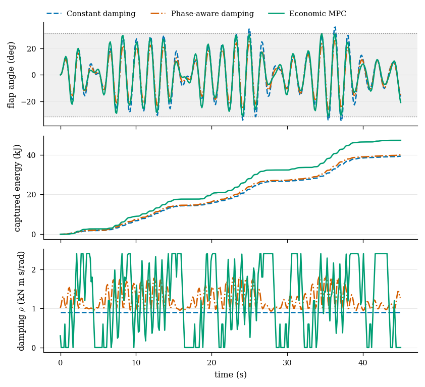
The economic MPC captures approximately 47.3 kJ, compared with 39.9 kJ for phase-aware damping and 39.3 kJ for constant damping. It reaches the 0.55 rad stroke limit and the 2.8 kN m torque limit without exceeding either beyond numerical tolerance. Constant damping exceeds the stroke limit by about 0.084 rad. The phase-aware law remains feasible and uses less damping variation, but it leaves energy unharvested.
One of the 375 nonlinear programs terminates without satisfying the solver’s convergence flag. The implementation then applies the shifted feasible sequence through the common actuator projection. The resulting trajectory remains within the recorded limits, but the fallback is part of the result rather than evidence of recursive feasibility.
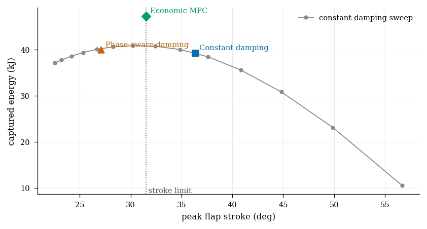
The constant-damping sweep places the three controllers on a common energy-motion diagram. A larger constant damping initially improves capture, then suppresses the motion that produces power. The economic MPC lies above this static tradeoff because it changes damping with the predicted phase while respecting the stroke bound.
Figure 2:Captured energy against peak flap stroke. Gray circles sweep constant passive damping from 100 to 2800 N m s/rad. The vertical dotted line is the 0.55 rad stroke constraint. Economic MPC obtains more energy than the fixed-damping sweep by scheduling damping over the predicted wave cycle. The phase-aware baseline is feasible but does not attain the MPC energy.
The animation shows the economic-MPC trajectory and accumulated energy from the same executed simulation. The displayed damping is the action applied after the actuator projection.
Figure 3:Time-compressed replay of the economic-MPC flap motion and captured energy. The controller re-solves an 18-step nonlinear program every 0.12 seconds and applies the first passive damping action.
Inspect the economic-MPC solve
1 2 3 4 5 6 7 8 9 10 11 12 13 14 15 16 17 18 19 20 21 22 23 24 25 26 27 28 29 30 31 32 33 34 35 36 37 38 39 40 41 42 43 44 45 46 47 48 49 50 51 52 53 54 55 56 57 58 59 60 61 62 63 64 65 66 67 68 69 70 71 72 73 74 75 76 77 78 79 80 81 82 83 84def solve_economic_mpc( time: float, state: np.ndarray, previous_damping: float, params: WaveParameters | None = None, *, warm_start: np.ndarray | None = None, max_iterations: int = 45, ) -> MPCStep: """Maximize predicted harvested energy under plant and actuator constraints.""" params = params or WaveParameters() params.validate() state = np.asarray(state, dtype=float) if state.shape != (2,) or not np.all(np.isfinite(state)): raise ValueError("state must have shape (2,) and contain finite values") horizon = params.horizon_steps if warm_start is None: initial = np.full(horizon, previous_damping, dtype=float) else: warm_start = np.asarray(warm_start, dtype=float) if warm_start.shape != (horizon,): raise ValueError("warm_start has the wrong horizon") initial = warm_start.copy() initial[0] = project_damping(initial[0], state[1], previous_damping, params) for k in range(1, horizon): change_limit = params.damping_rate_limit * params.control_period initial[k] = np.clip( initial[k], max(0.0, initial[k - 1] - change_limit), min(params.damping_max, initial[k - 1] + change_limit), ) def objective(normalized: np.ndarray) -> float: sequence = params.damping_max * normalized prediction = predict_trajectory(time, state, sequence, params) velocity = prediction[:-1, 1] energy = params.control_period * np.sum(sequence * velocity**2) changes = np.diff(np.concatenate([[previous_damping], sequence])) slew = np.sum((changes / params.damping_max) ** 2) return float(-energy / 1_000.0 + params.slew_weight * slew) def constraints(normalized: np.ndarray) -> np.ndarray: sequence = params.damping_max * normalized prediction = predict_trajectory(time, state, sequence, params) return _constraint_margins(sequence, prediction, previous_damping, params) started = perf_counter() result = minimize( objective, initial / params.damping_max, method="SLSQP", bounds=[(0.0, 1.0)] * horizon, constraints={"type": "ineq", "fun": constraints}, options={"maxiter": max_iterations, "ftol": 2e-6, "disp": False}, ) elapsed = perf_counter() - started sequence = np.asarray( params.damping_max * result.x if np.all(np.isfinite(result.x)) else initial ) prediction = predict_trajectory(time, state, sequence, params) margins = _constraint_margins(sequence, prediction, previous_damping, params) maximum_violation = float(max(0.0, -np.min(margins))) success = bool(result.success and maximum_violation <= 2e-4) if not success: sequence = initial prediction = predict_trajectory(time, state, sequence, params) margins = _constraint_margins(sequence, prediction, previous_damping, params) maximum_violation = float(max(0.0, -np.min(margins))) first = project_damping(sequence[0], state[1], previous_damping, params) sequence = sequence.copy() sequence[0] = first return MPCStep( damping=first, sequence=sequence, predicted_state=prediction, objective=float(objective(sequence / params.damping_max)), success=success, max_predicted_violation=maximum_violation, solve_time_s=elapsed, )
Download the complete wave-energy experiment
This model assumes an accurate short-term wave forecast and one rigid flap mode. Real devices include radiation-memory effects, additional structural modes, losses, measurement error, and forecast uncertainty. Those omissions affect both predicted capture and constraint margins. Robust or stochastic MPC can represent some of this uncertainty, while data can be used to estimate the unmodeled residual dynamics.
Robust MPC
How can feasibility and performance be protected against every disturbance in a bounded uncertainty set?
Some systems are exposed to external disturbances or small errors in the model. In those cases, we want the controller to make decisions that will still work no matter what happens, as long as the disturbances stay within some known bounds. This is the idea behind robust MPC.
Instead of planning a single trajectory, the controller plans a “nominal” path (what would happen in the absence of any disturbance) and then adds a feedback correction to react to whatever disturbances actually occur. This looks like:
where is the planned input and is a feedback gain that pulls the system back toward the nominal path if it deviates.
Because we know the worst-case size of the disturbance, we can estimate how far the real state might drift from the plan, and “shrink” the constraints accordingly. The result is that the nominal plan is kept safely away from constraint boundaries, so even if the system gets pushed around, it stays inside limits. This is often called tube MPC because the true trajectory stays inside a tube around the nominal one.
The main benefit is that we can handle uncertainty without solving a complicated worst-case optimization at every time step. All the uncertainty is accounted for in the design of the feedback and the tightened constraints.
Stochastic MPC
What becomes possible when uncertainty is represented by probabilities rather than only worst-case bounds?
If disturbances are random rather than adversarial, a natural goal is to optimize expected cost while enforcing constraints probabilistically. This gives rise to stochastic MPC, in which:
The cost becomes an expectation:
Constraints are allowed to be violated with small probability:
In practice, expectations are approximated using a finite set of disturbance scenarios drawn ahead of time. For each scenario, the system dynamics are simulated forward using the same control inputs , which are shared across all scenarios to respect non-anticipativity. The result is a single deterministic optimization problem with multiple parallel copies of the dynamics, one per sampled future. This retains the standard MPC structure, with only moderate growth in problem size.
Despite appearances, this is not dynamic programming. There is no value function or tree of all possible paths. There is only a finite set of futures chosen a priori, and optimized over directly. This scenario-based approach is common in energy systems such as hydro scheduling, where inflows are uncertain but sample trajectories can be generated from forecasts.
Risk constraints are typically enforced across all scenarios or encoded using risk measures like CVaR. For example, one might penalize violations that occur in the worst of samples, while still optimizing expected performance overall.
Hybrid and Mixed-Integer MPC
How can mode switches, on-off devices, and logical decisions enter the same finite-horizon optimization?
When systems involve discrete switches (eg. on/off valves, mode selection, or combinatorial logic) the MPC problem must include integer or binary variables. These show up in constraints like
where counts the binary decisions at each step, along with mode-dependent dynamics and costs. The resulting formulation is a mixed-integer nonlinear program (MINLP). The receding-horizon idea is the same, but each solve is more expensive due to the combinatorial nature of the decision space.
Distributed and Decentralized MPC
When one optimization is too large or ownership is distributed, which information must local controllers exchange to coordinate their plans?
Large-scale systems often consist of interacting subsystems. Distributed MPC decomposes the global NLP into smaller ones that run in parallel, with coordination constraints enforcing consistency across shared variables:
Each subsystem solves a local problem over its own state and input variables, then exchanges information with neighbors. Coordination can be done via primal–dual methods, ADMM, or consensus schemes, but each local block looks like a standard MPC problem.
Adaptive and Learning-Based MPC
How can the prediction model improve from data without discarding the explicit constraints enforced by MPC?
In practice, we may not know the true model or cost function precisely. In adaptive MPC, these are updated online from data:
The parameters and are learned in real time, and the subproblem solved at time uses their current estimates. When combined with policy distillation, value approximation, or trajectory imitation, this leads to overlaps with reinforcement learning where the MPC solutions act as supervision for a reactive policy.
Robustness and Failure Handling
What should the closed-loop system do when the preferred MPC problem is infeasible, inaccurate, or unfinished at the control deadline?
The wave-energy example assumes that every optimization finishes before the next control update and that its prediction model remains accurate over the horizon. An operational MPC controller must also handle incompatible constraints, modeling errors, and missed computation deadlines.
A disturbance can move the measured state to a point from which the requested target is unreachable within the horizon. Model mismatch can make a trajectory feasible in prediction and infeasible on the plant. A solver can also stop because of an ill-conditioned local model or a changing active set. These cases require an explicit hierarchy of hard constraints, soft objectives, and fallback actions. The following mechanisms modify the finite-horizon problem or its deployment without changing the receding-horizon principle.
Softening Constraints Through Slack Variables
Which constraints may be violated at a quantified price so that the optimizer can still return a usable action?
The first approach to handling infeasibility recognizes that not all constraints carry equal importance. A chemical reactor’s temperature must never exceed the runaway threshold: this is a hard constraint that cannot be violated. However, maintaining temperature within an optimal efficiency band is merely desirable. This can be treated as a soft constraint that we prefer to satisfy but can relax when necessary.
This hierarchy motivates reformulating the optimization problem using slack variables:
The penalty weights encode our priorities. Safety constraints might use , while comfort constraints use . This reformulated problem is always feasible as long as the hard constraints alone admit a solution. That is: we can always make the slack variables sufficiently large to satisfy the soft constraints.
Rather than treating constraints as binary hard/soft categories, we can establish a constraint hierarchy that enables graceful degradation:
As conditions deteriorate, the controller abandons objectives in reverse priority order, maintaining safety even when optimality becomes impossible.
Feasibility Restoration
If the main problem fails, can a secondary optimization recover a state from which the nominal constraints become satisfiable again?
When even soft constraints prove insufficient (perhaps due to catastrophic solver failure or corrupted problem structure) we need feasibility restoration that finds any feasible point regardless of optimality:
This formulation temporarily relaxes even the dynamics constraints, finding the “least infeasible” solution. It answers the question: if we must violate something, what is the minimal violation required? Once feasibility is restored, we can warm-start the original problem from this point.
Reference Governors
Can an unsafe reference be modified before it reaches an otherwise reliable inner controller?
Rather than reacting to infeasibility after it occurs, we can prevent it by filtering references through a reference governor. Consider an aircraft following waypoints. Instead of passing waypoints directly to the MPC, the governor asks: what is the closest approachable reference from our current state?
The governor performs a line search between the current state (always feasible since staying put requires no action) and the desired reference (potentially infeasible). This guarantees the MPC always receives feasible problems while making maximum progress toward the goal.
For computational efficiency, we can pre-compute the maximal output admissible set:
Online, the governor simply projects the desired reference onto .
Backup Controllers
Which independently validated action should take over when the optimizer or its model cannot be trusted?
When MPC fails entirely (due to solver crashes, timeouts, or numerical failures) we need backup controllers that require minimal computation while guaranteeing stability and keeping the system away from dangerous regions.
The standard approach uses a pre-computed local LQR controller around the equilibrium:
where are the linearized dynamics at equilibrium. When MPC fails:
The region represents the largest invariant set where LQR is guaranteed to work.
Cascade Architectures
How can slower optimization and faster local feedback be layered without giving both loops conflicting authority?
Production MPC systems rarely rely on a single solver. Instead, they implement a cascade of increasingly conservative controllers that trade optimality for reliability:
def get_control(self, x, time_budget):
    """
    Multi-level cascade for robust real-time control
    """
    time_remaining = time_budget

    # Level 1: Full nonlinear MPC
    if time_remaining > 5e-3:  # 5ms minimum
        try:
            u, solve_time = self.solve_nmpc(x, time_remaining)
            if converged:
                return u
        except:
            pass
        time_remaining -= solve_time

    # Level 2: Simplified linear MPC
    if time_remaining > 1e-3:  # 1ms minimum
        try:
            # Linearize around current state
            A, B = self.linearize_dynamics(x)
            u, solve_time = self.solve_lmpc(x, A, B, time_remaining)
            return u
        except:
            pass
        time_remaining -= solve_time

    # Level 3: Explicit MPC lookup
    if time_remaining > 1e-4:  # 0.1ms minimum
        region = self.find_critical_region(x)
        if region is not None:
            return self.explicit_control_law[region](x)

    # Level 4: LQR backup
    if self.in_lqr_region(x):
        return self.K_lqr @ (x - self.x_eq)

    # Level 5: Emergency safe mode
    return self.emergency_stop(x)
Each level trades optimality for reliability: Level 1 provides optimal but computationally expensive control, Level 2 offers suboptimal but faster solutions, Level 3 provides pre-computed instant evaluation, Level 4 ensures stabilizing control without tracking, and Level 5 implements safe shutdown.
Even when using backup controllers, we can maintain solution continuity through persistent warm-starting:
Here the superscript marks the solution computed at time , and subscripts remain prediction steps. The shift operation takes a successful MPC solution and moves it forward by one time step, appending a terminal action: . This shifted sequence provides natural temporal continuity for the next optimization.
When MPC fails and backup control is applied, the lift operation extends the single backup action into a full horizon-length sequence, either by repetition or by simulating the backup controller forward. This creates a reasonable warm-start guess from limited information.
The propagate operation maintains a “virtual” trajectory by continuing to evolve the previous solution as if it were still being executed, even when the actual system follows backup control. This forward simulation keeps the warm-start temporally aligned and relevant for when MPC recovers.
Inference Serving Under a Latency and Power Budget
How do deadlines, thermal limits, forecast error, and solver time interact in a receding-horizon controller for a real computing workload?
The offline frequency schedule in Trajectory Optimization cannot react when a burst arrives earlier than forecast. Receding-horizon control uses the same aggregate model but replaces the initial forecast after each second. Measured NVIDIA L4 service-rate and phase-power curves calibrate the model, while the request and queue trajectories remain simulation outputs. The scheduling rule remains fixed at the reduced 512-token interleaved chunked-prefill model from the modeling chapter, so the comparison isolates feedback through the GPU clock.
At control time , the state
contains queued prefill work, unfinished decode work, temperature, and the last applied clock. The controller forecasts ten one-second transitions. Arrivals are predicted from the trailing 30-second rate, while expected output work uses the empirical output-length distribution from the trace. The request-level plant receives the realized requests and output lengths instead.
The finite-horizon problem uses the normalized objective
where, as in the receding-horizon subproblem, counts seconds after the control time . The variables and are normalized overruns of two aggregate delay estimates. The first divides predicted queued prefill tokens by the profiled prefill rate. The second divides the predicted number of active decode requests by the profiled decode rate. These estimates enter the optimization but do not equal realized request-level TTFT and TPOT; the detailed simulation computes the latter. The frequency difference is normalized by the profiled clock range. The slacks and penalize violations of the experimental power and thermal limits, and penalizes unfinished work at the end of the horizon. SLSQP receives at most 50 iterations and a tolerance of 10-6. Only the first frequency is applied. The continuous result is rounded downward to the nearest profiled requested clock before the next state is observed. The replay reports the corresponding measured median realized clock separately, since the requested and realized values can differ under the experimental power cap.
A solver result is rejected if it is infeasible, non-finite, or arrives after the 0.8-second control budget. The fallback is a hysteretic reactive governor: it raises the clock by one profile level when weighted queue pressure reaches eight or the oldest prompt has waited one second, and lowers it by one level when temperature reaches 72 degrees C or pressure falls to one. Every fallback appears in the recorded trajectory rather than being removed from the aggregate metrics.
The comparison asks whether replanning improves the response to the shifted burst without hiding its energy cost. Four controllers receive identical requests and initial conditions:
maximum clock throughout the experiment;
the reactive governor used as the MPC fallback;
the open-loop schedule optimized for the nominal trace;
receding-horizon MPC.
Figure 4:Maximum-clock, reactive, open-loop, and MPC frequency control under the same shifted request trace and fixed reduced interleaved chunked-prefill model. Measured NVIDIA L4 curves calibrate each simulated trajectory. At each second, the dashed MPC segment is the current ten-second plan and the solid segment is the action history. Later plans are not revealed before they are computed.
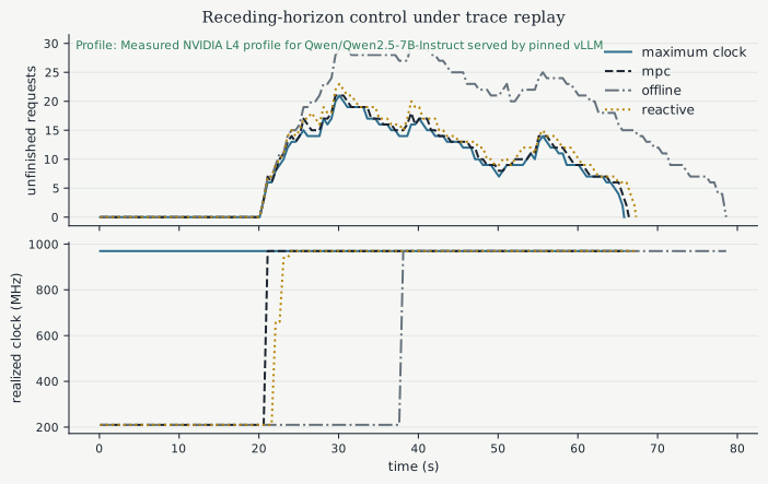
Figure 5:Static view of the closed-loop comparison. The online book provides playback and exposes the planned MPC horizon available at each control time.
The table compares the four frequency controllers under identical shifted arrivals and the fixed reduced interleaved chunked-prefill model. Fallback count records every MPC step that exceeded its feasibility, finiteness, or timing requirement.
Download every closed-loop metric (CSV)
On the shifted trace, maximum clock gives the lowest mean time to first token, 10.93 seconds, at 3,506.0 joules. Its 95th percentile is 18.41 seconds. MPC reduces energy to 3,341.8 joules, the lowest of the four controllers, while its mean and 95th-percentile times to first token are 11.53 and 19.01 seconds. The reactive governor records a mean of 12.51 seconds, a 95th percentile of 20.01 seconds, and 3,363.3 joules. The unchanged offline plan records 23.23 seconds, a 95th percentile of 31.28 seconds, and 3,646.8 joules.
Maximum clock and MPC both have a mean time per output token of 0.0417 seconds. The reactive governor records 0.0419 seconds, while the offline plan records 0.0466 seconds. The peak queue is 21 requests at maximum clock and 22 under MPC. It grows to 23 under the reactive governor and 30 under the offline plan. At the 60-second reporting horizon, maximum clock and MPC each leave nine requests unfinished. The reactive governor leaves 11, and the offline plan leaves 22. All 48 requests eventually complete during the post-horizon drain, whose energy is included in the reported totals.
Every controller violates the experimental TTFT limit for every request, and each has a 12.5% TPOT violation rate. MPC accepts 67 solves over the full rollout and invokes no fallback. Every accepted solve meets the 0.8-second deadline. On this trace, MPC improves both mean TTFT and energy relative to the reactive governor and the offline plan. Maximum clock remains 0.60 seconds faster in mean TTFT but consumes 164.2 joules more than MPC.
The displayed table focuses on latency, energy, queueing, constraint violations, and fallback count. The downloadable CSV also reports end-to-end latency, throughput, energy per output token, peak power and temperature, and unfinished work. The comparison therefore separates a faster response from a lower-energy response instead of assigning one score to each controller.
The measured profile supplies the service-rate and phase-power calibration; the controller trajectories are simulations of a single-GPU serving model. All four simulations reach a modeled phase power of 64.852 W at the highest requested clock. This value comes from the measured decode-phase mean for that profile level and is 0.052 W above the configured 64.800 W cap. The cap was an experimental setting rather than a hard sample-wise guarantee. None of the four simulations records a thermal or KV-capacity violation.
Live Comparison at Common Latency Targets
The live experiment asks which clock policy uses the least measured GPU energy while meeting common request-level latency limits. Development measurements select a fixed clock and set the limits on the 95th percentile of time to first token and of per-request mean inter-token latency. The planned confirmation compares this fixed clock, maximum clock, the governor, and MPC including its fallback. A constant clock or governor can be the preferred policy if it meets both limits with lower measured energy.
Development and confirmation each use 32 requests from disjoint portions of the recorded trace, under steady and bursty arrival schedules. Each arrival window spans at least 240 seconds. The GPU has a 40 W board power cap and a 6,251 MHz requested memory clock. Service rates and idle power require fresh measurements at this cap; the original 64.8 W calibration remains archived. The live state distinguishes requests awaiting their first output from requests already streaming. A transition model fitted on mixed-serving data must pass whole-run validation before it can support MPC. These measurements test queue drainage under the workload the controller will actually encounter.
Confirmation plans five paired repetitions per schedule across three independent acquisitions, with counterbalanced method order. Each pair uses identical requests and arrival times. Energy includes the final request drain; an efficiency claim requires all five valid pairs and both methods to meet both frozen latency limits. Invalid trials and fallback decisions remain in the record. Development qualification and a frozen comparison protocol are still needed before confirmation can begin.
Two earlier development acquisitions completed the full steady workload at 210 MHz, using 8.55 and 8.30 kJ, but could not return to their startup temperature references before the cooling timeout. A subsequent qualification warms the GPU with the full steady workload before selecting its reference from a stable 300-second cooling window. Its final 60-second mean fixes the reference for the remaining trials; this stability criterion does not establish thermal equilibrium.
That warm-reference acquisition qualified both requested settings, 210 and 660 MHz, on the two designated arrival patterns. All 32 requests completed validly in each of the four trials. The separate warm-up does not count toward qualification. Energy was 7.65 and 8.29 kJ for the 210 MHz bursty and steady trials, and 7.09 and 8.43 kJ for the corresponding 660 MHz trials. Clock labels name requested settings: the 660 MHz request produced lower measured clocks during active inference, with medians of 360 MHz for bursty and 300 MHz for steady arrivals. These operating-point checks establish neither a common latency target nor an energy winner. Controller development and a frozen comparison protocol are still required before confirmation.
Download the live experiment protocol and run instructions
Validation of the Thermal Constraint
The controller in the recorded replay constrains a junction temperature predicted by a one-state thermal model. None of the simulated controllers violates that constraint, but this establishes feasibility only for the model used inside the optimizer.
A power-matched pair of workloads exposes the modeling problem. During the held-out experiment, a 55 W decode pulse and a 55 W prefill pulse consumed nearly the same electrical energy, with a difference of 0.2 percent. The measured peak temperature rise during prefill was nevertheless 2.00 degrees C larger than during decode. A one-state model driven only by board power receives nearly the same input for both pulses and has no variable with which to represent this difference.
The clock sweep used to calibrate the serving model was designed to measure service rate and power. Its one-state thermal fit had , so a separate experiment tested whether workload phase was needed in the thermal input. Both candidate models used
Here is an effective ambient temperature, is the thermal time constant, and is the steady-state thermal resistance. The two input models differ by one term:
The indicator equals one during prefill and zero during decode. The phase-gain model can therefore assign different effective thermal inputs to two workloads with the same measured board power. Its state dimension and measured input remain unchanged.
The training and validation split used separate workload pulses:
| Data split | Workloads and duration | Use |
|---|---|---|
| Training | Decode and prefill at 46 W for 75 s and at 61 W for 45 s | Fit both candidate models |
| Validation | Decode and prefill at 55 W for 60 s | Evaluate the fixed models once |
The order of the four training pulses was counterbalanced. Every pulse began from a verified post-relock temperature within a one-degree-Celsius band. The acquisition retained a 77 degree C safe-down threshold and a 79 degree C abort threshold. Matching the measured junction temperature does not establish that the unobserved heat-sink temperature was also matched.
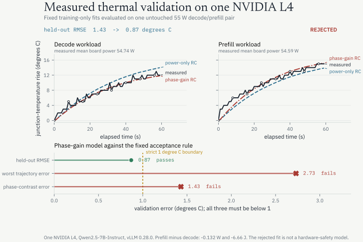
Figure 6:The power-only model predicts similar responses for the power-matched pulses. The phase-gain model separates them and lowers held-out RMSE, but its largest trajectory and phase-contrast errors remain above the fixed one-degree-Celsius acceptance boundary. The validation data were not used to fit either model.
On the held-out pair, the power-only model has an RMSE of 1.43 degrees C. Adding the workload-phase gain reduces this error to 0.87 degrees C. The fixed rule, however, requires all three validation errors to remain below 1 degree C. The phase-gain model reaches a worst trajectory error of 2.73 degrees C and a phase-contrast error of 1.43 degrees C, so the model is rejected.
The measured prefill peak rise exceeds the decode rise by 2.00 degrees C; the phase-gain model predicts a difference of 3.43 degrees C. Prefill draws 0.132 W less mean board power and consumes 6.66 J less energy than decode, with an energy ratio of 0.99797. Higher measured electrical input therefore cannot explain the larger prefill temperature rise in this pair.
These measurements come from one NVIDIA L4 serving Qwen2.5-7B-Instruct with vLLM 0.28.0. They do not establish a hardware-safety model or justify a mixed-serving thermal constraint.
The fitted gain gives prefill 1.147 times the effective thermal input of decode. This parameter is reproducible across the ten optimization starts. The training Jacobian also has full numerical rank, with condition number 384. These checks reduce concern about an ambiguous parameter fit, but they do not establish that one thermal state is sufficient. The validation residuals miss the rapid initial temperature rise and later reverse sign. Inherited thermal state, sensor timing and filtering, and phase-dependent heating remain possible explanations; these pulse measurements do not isolate their contributions.
Fitting the Complete Thermal History
The expanded development comparison selects a two-state thermal model. It adds the completed 4 September pilot, including its failed sustained-serving trial, to the five historical acquisitions. All six acquisitions, including the earlier validation data, are development data for this comparison.
Each acquisition retains its continuous temperature history through cooldown, memory relocking, and workload segments. The two-state model carries an unobserved heat-sink temperature through these transitions rather than resetting it to the measured junction temperature at each pulse. The fit compares predictions with the sensor’s one-degree-Celsius bins. Each evaluation holds out one complete acquisition; the table averages its ten-second RMSE equally across the six acquisitions. These predictions use measured future board power, so they test the temperature model with its future input supplied.
| Thermal model | Mean run-weighted ten-second RMSE (degrees C) |
|---|---|
| One state | 0.726 |
| One state with phase gain, diagnostic only | 0.722 |
| Two states | 0.540 |
| Two states with phase gain, diagnostic only | 0.518 |
The unchanged selection rule requires at least 0.1 degrees C and a ten-percent improvement to add a state, without materially worsening one-second error or ten-second underprediction. The two-state model improves mean RMSE by 0.186 degrees C, or 25.58 percent, and passes those safeguards. Its fitted modes are about 1.72 and 154 seconds. These describe the model response under the recorded sensor alignment; they do not establish uniquely identified physical time constants. Phase-gain models remain diagnostic because mixed serving supplies no runtime phase-activity signal.
The gain is smaller within the failed sustained trial: ten-second RMSE falls from 0.907 to 0.825 degrees C across only nine forecast origins. The raw sensor peak is 77 degrees C, while the retained one-second observations peak at 76. The selected model was frozen before the 40 W acquisition. Fresh evaluation still needs power forecasts available when the controller acts. The model remains unaccepted for online advisory forecasts or hard thermal constraints; measured-temperature watchdogs operate independently.
Download the six-acquisition thermal development report (JSON)
The original five-acquisition analysis retained one state because adding a second state improved RMSE by only 0.069 degrees C, below the same absolute threshold. Its data and report remain unchanged.
Download the original five-acquisition report (JSON)
For the recorded MPC simulation, the temperature state and inequality remain a teaching model. The absence of a simulated thermal violation is not a hardware safety certificate. The arrival forecast is deliberately simple, output length is observed only at completion, and the scheduler is held fixed. Network delay, tokenization, multi-GPU communication, and model-quality effects are omitted. The shifted burst is one controlled disturbance, so relative performance on that trace does not establish dominance under other workloads.
Download the one-second held-out trajectories and fixed-model predictions (CSV)
Download the complete thermal fit and acceptance report (JSON)
Download the measured validation telemetry (CSV)
Inspect the receding-horizon controller
1 2 3 4 5 6 7 8 9 10 11 12 13 14 15 16 17 18 19 20 21 22 23 24 25 26 27 28 29 30 31 32 33 34 35 36 37 38 39 40 41 42 43 44 45 46 47 48 49 50 51 52 53 54 55 56 57 58 59 60 61 62 63 64 65 66 67 68 69 70 71 72 73 74 75 76 77 78 79 80 81 82 83 84def _solve(self, observation: ServingObservation, arrival_rate: float) -> tuple[np.ndarray, bool, float]: profile = self.plant.profile minimum = profile.minimum_clock_mhz maximum = profile.maximum_clock_mhz initial_prefill_tokens = observation.prefill_remaining_tokens initial_decode_tokens = estimate_decode_remaining_tokens( observation.decode_active, observation.generated_decode_tokens, self.mean_output_tokens, ) prompt_arrivals = np.full( self.horizon_steps, arrival_rate * self.mean_prompt_tokens * self.control_period_s, ) initial = np.full(self.horizon_steps, self.current_clock) maximum_power = max(profile.prefill_power_w[-1], profile.decode_power_w[-1]) def objective(sequence: np.ndarray) -> float: ( prefill_tokens, decode_tokens, active_decode, temperature, normalized_power, ttft_proxy, tpot_proxy, ) = _mpc_fluid_rollout( sequence, initial_prefill_tokens=initial_prefill_tokens, initial_decode_tokens=initial_decode_tokens, initial_active_decode=float(observation.decode_active), prompt_arrivals=prompt_arrivals, mean_prompt_tokens=self.mean_prompt_tokens, mean_output_tokens=self.mean_output_tokens, plant=self.plant, control_period_s=self.control_period_s, initial_temperature_c=observation.temperature_c, ) normalized_frequency = (sequence - minimum) / (maximum - minimum) previous_normalized = (self.current_clock - minimum) / (maximum - minimum) changes = np.diff( np.concatenate([[previous_normalized], normalized_frequency]) ) ttft_slack = np.maximum(0.0, ttft_proxy - profile.ttft_slo_s) / max( profile.ttft_slo_s, 1e-12 ) tpot_slack = np.maximum( 0.0, tpot_proxy - profile.tpot_slo_s, ) / max(profile.tpot_slo_s, 1e-12) power_slack = np.maximum( 0.0, normalized_power - self.plant.power_limit_w / maximum_power, ) thermal_slack = np.maximum(0.0, temperature[1:] - self.plant.thermal_limit_c) terminal_backlog = ( prefill_tokens[-1] / profile.prefill_tokens_per_s[-1] + decode_tokens[-1] / profile.decode_tokens_per_s[-1] ) return float( np.sum(normalized_power) + 20.0 * np.sum(ttft_slack**2) + 10.0 * np.sum(tpot_slack**2) + 0.05 * np.sum(changes**2) + 1_000.0 * np.sum(power_slack**2 + thermal_slack**2) + 20.0 * terminal_backlog**2 ) start = perf_counter() solution = minimize( objective, initial, method="SLSQP", bounds=[(minimum, maximum)] * self.horizon_steps, options={"maxiter": 50, "ftol": 1e-6, "disp": False}, ) elapsed = perf_counter() - start candidate = np.asarray(solution.x, dtype=float) success = bool( solution.success and np.all(np.isfinite(candidate)) and elapsed <= self.solve_time_limit_s ) return candidate, success, elapsed
1 2 3 4 5 6 7 8 9 10 11 12 13 14 15 16 17 18 19 20 21 22 23 24 25 26 27 28 29def run_mpc( workload: Sequence[Request], plant: ServingPlant, scheduler: Scheduler = chunked_prefill_scheduler, *, horizon_s: float = 10.0, control_period_s: float = 1.0, solve_time_limit_s: float = 0.8, seed: int = 0, ) -> ServingResult: """Run receding-horizon frequency control on the detailed plant.""" controller = _MPCClockController( workload, plant, horizon_s=horizon_s, control_period_s=control_period_s, solve_time_limit_s=solve_time_limit_s, ) return simulate( workload, plant, scheduler, controller, seed, controller_name="MPC", scheduler_name="512-token interleaved chunked-prefill surrogate", )
Summary and Outlook
Tracking, regulation, economic control, robustness, stochastic predictions, and hybrid decisions all retain the same receding-horizon backbone while changing the objective, uncertainty model, or feasible set. Slack variables, reference governors, backup controllers, and cascades determine how the controller behaves when the preferred optimization problem is late or infeasible.
Reliable execution still requires solving a closely related optimization problem at every step. Can repeated structure be reused, or even approximated by a learned map from parameters to actions? Parametric and approximate controllers develop those alternatives.
Self-checks
Solution to Exercise 1
The decision is computed for the state at the start of a one-second interval. After the deadline, little time remains to apply it and the request queue may already have changed. The reactive fallback supplies a timely action with known bounds.
Solution to Exercise 2
No. A reproducible parameter estimate does not establish that the model class captures the relevant plant dynamics. The failed held-out criterion prevents the constraint from serving as a safety certificate. The experiment remains useful because it measures a discrepancy between power-matched workloads and quantifies the prediction improvement from a phase-dependent input. It does not identify the physical cause: inherited thermal state and sensor timing or filtering remain competing explanations to test with complete acquisition histories.