Model Predictive Control#
The trajectory optimization methods presented so far compute a complete control trajectory from an initial state to a final time or state. Once computed, this trajectory is executed without modification, making these methods fundamentally open-loop. The control function, \(\mathbf{u}[k]\) in discrete time or \(\mathbf{u}(t)\) in continuous time, depends only on the clock, reading off precomputed values from memory or interpolating between them. This approach assumes perfect models and no disturbances. Under these idealized conditions, repeating the same control sequence from the same initial state would always produce identical results.
Real systems face modeling errors, external disturbances, and measurement noise that accumulate over time. A precomputed trajectory becomes increasingly irrelevant as these perturbations push the actual system state away from the predicted path. The solution is to incorporate feedback, making control decisions that respond to the current state rather than blindly following a predetermined schedule. While dynamic programming provides the theoretical framework for deriving feedback policies through value functions and Bellman equations, there exists a more direct approach that leverages the trajectory optimization methods already developed.
Closing the Loop by Replanning#
Model Predictive Control creates a feedback controller by repeatedly solving trajectory optimization problems. Rather than computing a single trajectory for the entire task duration, MPC solves a finite-horizon problem at each time step, starting from the current measured state. The controller then applies only the first control action from this solution before repeating the entire process. This strategy transforms any trajectory optimization method into a feedback controller.
The Receding Horizon Principle#
The defining characteristic of MPC is its receding horizon strategy. At each time step, the controller solves an optimization problem looking a fixed duration into the future, but this prediction window constantly moves forward in time. The horizon “recedes” because it always starts from the current time and extends forward by the same amount.
Consider the discrete-time optimal control problem in Bolza form:
At time step \(t\), this problem optimizes over the interval \([t, t+N]\). At the next time step \(t+1\), the horizon shifts to \([t+1, t+N+1]\). The key insight is that only the first control \(\mathbf{u}_0^*\) from each optimization is applied. The remaining controls \(\mathbf{u}_1^*, \ldots, \mathbf{u}_{N-1}^*\) are discarded, though they may initialize the next optimization through warm-starting.
This receding horizon principle enables feedback without computing an explicit policy. By constantly updating predictions based on current measurements, MPC naturally corrects for disturbances and model errors. The apparent waste of computing but not using most of the trajectory is actually the mechanism that provides robustness.
Horizon Selection and Problem Formulation#
The choice of prediction horizon depends on the control objective. We distinguish between three cases, each requiring different mathematical formulations.
Infinite-Horizon Regulation#
For stabilization problems where the system must operate indefinitely around an equilibrium, the true objective is:
Since this cannot be solved directly, MPC approximates it with:
The terminal cost \(V_f(\mathbf{x}_N)\) approximates \(\sum_{k=N}^{\infty} c(\mathbf{x}_k, \mathbf{u}_k)\), the cost-to-go beyond the horizon. The terminal constraint \(\mathbf{x}_N \in \mathcal{X}_f\) ensures the state reaches a region where a known stabilizing controller exists. Without these terminal ingredients, the finite-horizon approximation may produce unstable behavior, as the controller ignores consequences beyond the horizon.
Finite-Duration Tasks#
For tasks ending at time \(t_f\), the true objective spans from current time \(t\) to \(t_f\):
The MPC formulation must adapt as time progresses:
As the task approaches completion, the horizon shrinks and the terminal cost switches from the approximation \(c_T\) to the true final cost \(c_f\). This prevents the controller from optimizing beyond task completion, which would produce meaningless or aggressive control actions.
Periodic Tasks#
Some systems operate on repeating cycles where the optimal behavior depends on the time of day, week, or season. Consider a commercial building where heating costs are higher at night, electricity prices vary hourly, and occupancy patterns repeat daily. The MPC controller must account for these periodic patterns while planning over a finite horizon.
For tasks with period \(T_p\), such as daily building operations, the formulation accounts for transitions across period boundaries:
The cost function changes based on the phase \(\phi\) within the period. Constraints may similarly depend on the phase, reflecting different operational requirements at different times.
The MPC Algorithm#
The complete MPC procedure implements the receding horizon principle through repeated optimization:
Algorithm 2 (Model Predictive Control with Horizon Management)
Input:
Nominal prediction horizon \(N\)
Sampling period \(\Delta t\)
Task type: {infinite, finite with duration \(t_f\), periodic with period \(T_p\)}
Cost functions and dynamics
Constraints
Procedure:
Initialize time \(t \leftarrow 0\)
Measure initial state \(\mathbf{x}_{\text{current}} \leftarrow \mathbf{x}(t)\)
While task continues:
Determine effective horizon and costs:
If infinite task:
\(N_{\text{eff}} \leftarrow N\)
Use terminal cost \(V_f\) and constraint \(\mathcal{X}_f\)
If finite task:
\(N_{\text{eff}} \leftarrow \min(N, \lfloor(t_f - t)/\Delta t\rfloor)\)
If \(t + N_{\text{eff}}\Delta t = t_f\): use final cost \(c_f\)
Otherwise: use approximation \(c_T\)
If periodic task:
\(N_{\text{eff}} \leftarrow N\)
Adjust costs/constraints based on phase
Solve optimization: Minimize over \(\mathbf{u}_{0:N_{\text{eff}}-1}\) subject to dynamics, constraints, and \(\mathbf{x}_0 = \mathbf{x}_{\text{current}}\)
Apply receding horizon control:
Extract \(\mathbf{u}^*_0\) from solution
Apply to system for duration \(\Delta t\)
Measure new state
Advance time: \(t \leftarrow t + \Delta t\)
End While
Successive Linearization and Quadratic Approximations#
For many regulation and tracking problems, the nonlinear dynamics and costs we encounter can be approximated locally by linear and quadratic functions. The basic idea is to linearize the system around the current operating point and approximate the cost with a quadratic form. This reduces each MPC subproblem to a quadratic program (QP), which can be solved reliably and very quickly using standard solvers.
Suppose the true dynamics are nonlinear,
Around a nominal trajectory \((\bar{\mathbf{x}}_k,\bar{\mathbf{u}}_k)\), we take a first-order expansion:
with Jacobians
Similarly, if the stage cost is nonlinear,
we approximate it quadratically near the nominal point:
with positive semidefinite weighting matrices \(\mathbf{Q}_k\) and \(\mathbf{R}_k\).
The resulting MPC subproblem has the form
where \(\mathbf{d}_k = f(\bar{\mathbf{x}}_k,\bar{\mathbf{u}}_k) - \mathbf{A}_k \bar{\mathbf{x}}_k - \mathbf{B}_k \bar{\mathbf{u}}_k\) captures the local affine offset.
Because the dynamics are now linear and the cost quadratic, this optimization problem is a convex quadratic program. Quadratic programs are attractive in practice: they can be solved at kilohertz rates with mature numerical methods, making them the backbone of many real-time MPC implementations.
At each MPC step, the controller updates its linearization around the new operating point, constructs the local QP, and solves it. The process repeats, with the linear model and quadratic cost refreshed at every reoptimization. Despite the approximation, this yields a closed-loop controller that inherits the fast computation of QPs while retaining the ability to track trajectories of the underlying nonlinear system.
Theoretical Guarantees#
The finite-horizon approximation in MPC brings a new challenge: the controller cannot see consequences beyond the horizon. Without proper design, this myopia can destabilize even simple systems. The solution is to carefully encode information about the infinite-horizon problem into the finite-horizon optimization through its terminal conditions.
Before diving into the mathematics, we must clarify what “stability” means and which tasks these theoretical guarantees address, as the notion of stability varies significantly across different control objectives.
Stability Notions Across Control Tasks#
The terminal conditions provide different types of guarantees depending on the control objective. For regulation problems, where the task is to drive the state to a fixed equilibrium \((\mathbf{x}_\mathrm{eq}, \mathbf{u}_\mathrm{eq})\) (often shifted to the origin), the stability guarantee is asymptotic stability: starting sufficiently close to the equilibrium, we have \(\mathbf{x}_k \to \mathbf{x}_\mathrm{eq}\) while constraints remain satisfied throughout the trajectory (recursive feasibility). This requires the stage cost \(\ell(\mathbf{x},\mathbf{u})\) to be positive definite in the deviation from equilibrium.
When tracking a constant setpoint, the task becomes following a constant reference \((\mathbf{x}_\mathrm{ref},\mathbf{u}_\mathrm{ref})\) that solves the steady-state equations. This problem is handled by working in error coordinates \(\tilde{\mathbf{x}}=\mathbf{x}-\mathbf{x}_\mathrm{ref}\) and \(\tilde{\mathbf{u}}=\mathbf{u}-\mathbf{u}_\mathrm{ref}\), transforming the tracking problem into a regulation problem for the error system. The stability guarantee becomes asymptotic tracking, meaning \(\tilde{\mathbf{x}}_k \to 0\), again with recursive feasibility.
The terminal conditions we discuss below primarily address regulation and constant reference tracking. Time-varying tracking and economic MPC require additional techniques such as tube MPC and dissipativity theory.
MPC with Stability Guarantees#
To provide theoretical guarantees, the finite-horizon MPC problem is augmented with three interconnected components. The terminal cost \(V_f(\mathbf{x})\) approximates the cost-to-go beyond the horizon, providing a surrogate for the infinite-horizon tail that cannot be explicitly optimized. The terminal constraint set \(\mathcal{X}_f\) defines a region where we have local knowledge of how to stabilize the system. Finally, the terminal controller \(\kappa_f(\mathbf{x})\) provides a local stabilizing control law that remains valid within \(\mathcal{X}_f\).
These components must satisfy specific compatibility conditions to provide theoretical guarantees:
Theorem 1 (Recursive Feasibility and Asymptotic Stability)
Consider the MPC problem with terminal cost \(V_f\), terminal set \(\mathcal{X}_f\), and local controller \(\kappa_f\). If the following conditions hold:
Control invariance: For all \(\mathbf{x} \in \mathcal{X}_f\), we have \(\mathbf{f}(\mathbf{x}, \kappa_f(\mathbf{x})) \in \mathcal{X}_f\) (the set is invariant) and \(\mathbf{g}(\mathbf{x}, \kappa_f(\mathbf{x})) \leq \mathbf{0}\) (constraints remain satisfied).
Lyapunov decrease: For all \(\mathbf{x} \in \mathcal{X}_f\):
where \(\ell\) is the stage cost.
Then the MPC controller achieves recursive feasibility (if the problem is feasible at time \(k\), it remains feasible at time \(k+1\)), asymptotic stability to the target equilibrium for regulation problems, and monotonic cost decrease along trajectories until the target is reached.
Suboptimality Bounds#
The finite-horizon MPC value \(V_N(\mathbf{x})\) provides an upper bound approximation of the true infinite-horizon value \(V_\infty(\mathbf{x})\). Understanding how close this approximation can be reveals fundamental insights about the effectiveness of short-horizon MPC.
The upper bound \(V_N(\mathbf{x}) \geq V_\infty(\mathbf{x})\) follows immediately from the fact that MPC considers fewer control choices. The infinite-horizon controller can choose any sequence \((\mathbf{u}_0, \mathbf{u}_1, \mathbf{u}_2, \ldots)\), while the \(N\)-horizon controller is restricted to sequences of the form \((\mathbf{u}_0, \ldots, \mathbf{u}_{N-1}, \kappa_f(\mathbf{x}_N), \kappa_f(\mathbf{x}_{N+1}), \ldots)\) where the tail follows the fixed terminal controller. Since the infinite-horizon problem optimizes over a larger feasible set, its optimal value cannot exceed that of the finite-horizon problem.
Deriving the Approximation Error#
The interesting question is bounding the approximation error \(\varepsilon_N = V_N(\mathbf{x}) - V_\infty(\mathbf{x})\). This error represents the cost of being forced to use \(\kappa_f\) beyond the horizon rather than continuing to optimize.
Let \((\mathbf{u}_0^*, \mathbf{u}_1^*, \ldots)\) denote the infinite-horizon optimal control sequence with corresponding state trajectory \((\mathbf{x}_0^*, \mathbf{x}_1^*, \ldots)\) where \(\mathbf{x}_0^* = \mathbf{x}\). The infinite-horizon cost is:
Now consider what happens when we truncate this optimal sequence at horizon \(N\) and continue with the terminal controller. The cost becomes:
where \(V_f(\mathbf{x}_N^*)\) approximates the tail cost \(\sum_{k=N}^{\infty} \ell(\mathbf{x}_k^*, \mathbf{u}_k^*)\).
Since \(V_N(\mathbf{x})\) is the optimal \(N\)-horizon cost (which may do better than this particular truncated sequence), we have \(V_N(\mathbf{x}) \leq \tilde{V}_N(\mathbf{x})\). The approximation error therefore satisfies:
This bound reveals that the approximation error depends on how well the terminal cost \(V_f\) approximates the true tail cost along the infinite-horizon optimal trajectory.
The Landscape of MPC Variants#
Once the basic idea of receding-horizon control is clear, it is helpful to see how the same backbone accommodates many variations. In every case, we transcribe the continuous-time optimal control problem into a nonlinear program of the form
The components in this NLP come from discretizing the continuous-time problem with a fixed horizon \([t, t+T]\) and step size \(\Delta t\). The stage weights \(w_k\) and discrete dynamics \(\mathbf{F}_k\) are determined by the choice of quadrature and integration scheme. With this blueprint in place, the rest is a matter of interpretation: how we define the cost, how we handle uncertainty, how we treat constraints, and what structure we exploit.
Tracking MPC#
The most common setup is reference tracking. Here, we are given time-varying target trajectories \((\mathbf{x}_k^{\text{ref}}, \mathbf{u}_k^{\text{ref}})\), and the controller’s job is to keep the system close to these. The cost is typically quadratic:
When dynamics are linear and constraints are polyhedral, this yields a convex quadratic program at each time step.
Regulatory MPC#
In regulation tasks, we aim to bring the system back to an equilibrium point \((\mathbf{x}^e, \mathbf{u}^e)\), typically in the presence of disturbances. This is simply tracking MPC with constant references:
To guarantee stability, it is common to include a terminal constraint \(\mathbf{x}_N \in \mathcal{X}_f\), where \(\mathcal{X}_f\) is a control-invariant set under a known feedback law.
Economic MPC#
Not all systems operate around a reference. Sometimes the goal is to optimize a true economic objective (eg. energy cost, revenue, efficiency) directly. This gives rise to economic MPC, where the cost functions reflect real operational performance:
There is no reference trajectory here. The optimal behavior emerges from the cost itself. In this setting, standard stability arguments no longer apply automatically, and one must be careful to add terminal penalties or constraints that ensure the closed-loop system remains well-behaved.
Robust MPC#
Some systems are exposed to external disturbances or small errors in the model. In those cases, we want the controller to make decisions that will still work no matter what happens, as long as the disturbances stay within some known bounds. This is the idea behind robust MPC.
Instead of planning a single trajectory, the controller plans a “nominal” path (what would happen in the absence of any disturbance) and then adds a feedback correction to react to whatever disturbances actually occur. This looks like:
where \(\bar{\mathbf{u}}_k\) is the planned input and \(\mathbf{K}\) is a feedback gain that pulls the system back toward the nominal path if it deviates.
Because we know the worst-case size of the disturbance, we can estimate how far the real state might drift from the plan, and “shrink” the constraints accordingly. The result is that the nominal plan is kept safely away from constraint boundaries, so even if the system gets pushed around, it stays inside limits. This is often called tube MPC because the true trajectory stays inside a tube around the nominal one.
The main benefit is that we can handle uncertainty without solving a complicated worst-case optimization at every time step. All the uncertainty is accounted for in the design of the feedback \(\mathbf{K}\) and the tightened constraints.
Stochastic MPC#
If disturbances are random rather than adversarial, a natural goal is to optimize expected cost while enforcing constraints probabilistically. This gives rise to stochastic MPC, in which:
The cost becomes an expectation:
\[ \mathbb{E} \left[ c(\mathbf{x}_N) + \sum_{k=0}^{N-1} w_k\, c(\mathbf{x}_k, \mathbf{u}_k) \right] \]Constraints are allowed to be violated with small probability:
\[ \mathbb{P}[\mathbf{g}(\mathbf{x}_k, \mathbf{u}_k) \leq \mathbf{0}] \geq 1 - \varepsilon \]
In practice, expectations are approximated using a finite set of disturbance scenarios drawn ahead of time. For each scenario, the system dynamics are simulated forward using the same control inputs \(\mathbf{u}_k\), which are shared across all scenarios to respect non-anticipativity. The result is a single deterministic optimization problem with multiple parallel copies of the dynamics, one per sampled future. This retains the standard MPC structure, with only moderate growth in problem size.
Despite appearances, this is not dynamic programming. There is no value function or tree of all possible paths. There is only a finite set of futures chosen a priori, and optimized over directly. This scenario-based approach is common in energy systems such as hydro scheduling, where inflows are uncertain but sample trajectories can be generated from forecasts.
Risk constraints are typically enforced across all scenarios or encoded using risk measures like CVaR. For example, one might penalize violations that occur in the worst \((1 - \alpha)\%\) of samples, while still optimizing expected performance overall.
Hybrid and Mixed-Integer MPC#
When systems involve discrete switches (eg. on/off valves, mode selection, or combinatorial logic) the MPC problem must include integer or binary variables. These show up in constraints like
along with mode-dependent dynamics and costs. The resulting formulation is a mixed-integer nonlinear program (MINLP). The receding-horizon idea is the same, but each solve is more expensive due to the combinatorial nature of the decision space.
Distributed and Decentralized MPC#
Large-scale systems often consist of interacting subsystems. Distributed MPC decomposes the global NLP into smaller ones that run in parallel, with coordination constraints enforcing consistency across shared variables:
Each subsystem solves a local problem over its own state and input variables, then exchanges information with neighbors. Coordination can be done via primal–dual methods, ADMM, or consensus schemes, but each local block looks like a standard MPC problem.
Adaptive and Learning-Based MPC#
In practice, we may not know the true model \(\mathbf{F}_k\) or cost function \(c\) precisely. In adaptive MPC, these are updated online from data:
The parameters \(\boldsymbol{\theta}_t\) and \(\boldsymbol{\phi}_t\) are learned in real time. When combined with policy distillation, value approximation, or trajectory imitation, this leads to overlaps with reinforcement learning where the MPC solutions act as supervision for a reactive policy.
Robustness in Real-Time MPC#
The trajectory optimization methods we have studied assume perfect models and deterministic dynamics. In practice, however, MPC controllers must operate in environments where models are approximate, disturbances are unpredictable, and computational resources are limited. The mathematical elegance of optimal control must always yield to the engineering reality of robust operation as perfect optimality is less important than reliable operation. This philosophy permeates industrial MPC applications. A controller that achieves 95% performance 100% of the time is superior to one that achieves 100% performance 95% of the time and fails catastrophically the remaining 5%. Airlines accept suboptimal fuel consumption over missed approaches, power grids tolerate efficiency losses to prevent blackouts, and chemical plants sacrifice yield for safety. By designing for failure, we want to to create MPC systems that degrade gracefully rather than fail catastrophically, maintaining safety and stability even when the impossible is asked of them.
Example: Wind Farm Yield Optimization#
Consider a wind farm where MPC controllers coordinate individual turbines to maximize overall power production while minimizing wake interference. Each turbine can adjust both its thrust coefficient (through blade pitch) and yaw angle to redirect its wake away from downstream turbines. At time \(t_k\), the MPC controller solves the optimization problem:
Now suppose an unexpected wind direction change occurs, shifting the incoming wind vector by 30 degrees. The current state \(\mathbf{x}_{\text{current}}\) reflects wake patterns that no longer align with the new wind direction, and the optimizer discovers that no feasible trajectory exists that can redirect all wakes appropriately within the physical limits of yaw rate and thrust adjustment. The solver reports infeasibility.
This scenario reveals the fundamental challenge of real-time MPC: constraint incompatibility. When disturbances push the system into states from which recovery appears impossible, or when reference trajectories demand physically impossible maneuvers, the intersection of all constraint sets becomes empty. Model mismatch compounds this problem as prediction errors accumulate over the horizon.
Even when feasible solutions exist, computational constraints can prevent their discovery. A control loop running at 100 Hz allows only 10 milliseconds per iteration. If the solver requires 15 milliseconds to converge, we face an impossible choice: delay the control action and risk destabilizing the system, or apply an unconverged iterate that may violate critical constraints.
A third failure mode involves numerical instabilities: ill-conditioned matrices, rank deficiency, or division by zero in the linear algebra routines. These failures are particularly problematic because they occur sporadically, triggered by specific state configurations that create near-singular conditions in the optimization problem.
Softening Constraints Through Slack Variables#
The first approach to handling infeasibility recognizes that not all constraints carry equal importance. A chemical reactor’s temperature must never exceed the runaway threshold: this is a hard constraint that cannot be violated. However, maintaining temperature within an optimal efficiency band is merely desirable. This can be treated as a soft constraint that we prefer to satisfy but can relax when necessary.
This hierarchy motivates reformulating the optimization problem using slack variables:
The penalty weights \(\boldsymbol{\rho}\) encode our priorities. Safety constraints might use \(\rho_j = 10^6\), while comfort constraints use \(\rho_j = 1\). This reformulated problem is always feasible as long as the hard constraints alone admit a solution. That is: we can always make the slack variables \(\boldsymbol{\epsilon}\) sufficiently large to satisfy the soft constraints.
Rather than treating constraints as binary hard/soft categories, we can establish a constraint hierarchy that enables graceful degradation:
As conditions deteriorate, the controller abandons objectives in reverse priority order, maintaining safety even when optimality becomes impossible.
Feasibility Restoration#
When even soft constraints prove insufficient (perhaps due to catastrophic solver failure or corrupted problem structure) we need feasibility restoration that finds any feasible point regardless of optimality:
This formulation temporarily relaxes even the dynamics constraints, finding the “least infeasible” solution. It answers the question: if we must violate something, what is the minimal violation required? Once feasibility is restored, we can warm-start the original problem from this point.
Reference Governors#
Rather than reacting to infeasibility after it occurs, we can prevent it by filtering references through a reference governor. Consider an aircraft following waypoints. Instead of passing waypoints directly to the MPC, the governor asks: what is the closest approachable reference from our current state?
The governor performs a line search between the current state (always feasible since staying put requires no action) and the desired reference (potentially infeasible). This guarantees the MPC always receives feasible problems while making maximum progress toward the goal.
For computational efficiency, we can pre-compute the maximal output admissible set:
Online, the governor simply projects the desired reference onto \(\mathcal{O}_\infty\).
Backup Controllers#
When MPC fails entirely (due to solver crashes, timeouts, or numerical failures) we need backup controllers that require minimal computation while guaranteeing stability and keeping the system away from dangerous regions.
The standard approach uses a pre-computed local LQR controller around the equilibrium:
where \((\mathbf{A}, \mathbf{B})\) are the linearized dynamics at equilibrium. When MPC fails:
The region \(\mathcal{X}_{\text{LQR}} = \{\mathbf{x} : (\mathbf{x} - \mathbf{x}_{\text{eq}})^T \mathbf{P} (\mathbf{x} - \mathbf{x}_{\text{eq}}) \leq \alpha\}\) represents the largest invariant set where LQR is guaranteed to work.
Cascade Architectures#
Production MPC systems rarely rely on a single solver. Instead, they implement a cascade of increasingly conservative controllers that trade optimality for reliability:
def get_control(self, x, time_budget):
    """
    Multi-level cascade for robust real-time control
    """
    time_remaining = time_budget

    # Level 1: Full nonlinear MPC
    if time_remaining > 5e-3:  # 5ms minimum
        try:
            u, solve_time = self.solve_nmpc(x, time_remaining)
            if converged:
                return u
        except:
            pass
        time_remaining -= solve_time

    # Level 2: Simplified linear MPC
    if time_remaining > 1e-3:  # 1ms minimum
        try:
            # Linearize around current state
            A, B = self.linearize_dynamics(x)
            u, solve_time = self.solve_lmpc(x, A, B, time_remaining)
            return u
        except:
            pass
        time_remaining -= solve_time

    # Level 3: Explicit MPC lookup
    if time_remaining > 1e-4:  # 0.1ms minimum
        region = self.find_critical_region(x)
        if region is not None:
            return self.explicit_control_law[region](x)

    # Level 4: LQR backup
    if self.in_lqr_region(x):
        return self.K_lqr @ (x - self.x_eq)

    # Level 5: Emergency safe mode
    return self.emergency_stop(x)
Each level trades optimality for reliability: Level 1 provides optimal but computationally expensive control, Level 2 offers suboptimal but faster solutions, Level 3 provides pre-computed instant evaluation, Level 4 ensures stabilizing control without tracking, and Level 5 implements safe shutdown.
Even when using backup controllers, we can maintain solution continuity through persistent warm-starting:
The shift operation takes a successful MPC solution and moves it forward by one time step, appending a terminal action: \([\mathbf{u}_1^{(k)}, \mathbf{u}_2^{(k)}, \ldots, \mathbf{u}_{N-1}^{(k)}, \kappa_f(\mathbf{x}_N^{(k)})]\). This shifted sequence provides natural temporal continuity for the next optimization.
When MPC fails and backup control is applied, the lift operation extends the single backup action \(\mathbf{u}_{\text{backup}}^{(k)}\) into a full horizon-length sequence, either by repetition or by simulating the backup controller forward. This creates a reasonable warm-start guess from limited information.
The propagate operation maintains a “virtual” trajectory by continuing to evolve the previous solution as if it were still being executed, even when the actual system follows backup control. This forward simulation keeps the warm-start temporally aligned and relevant for when MPC recovers.
Example: Chemical Reactor Control Under Failure#
Consider a continuous stirred tank reactor (CSTR) where an exothermic reaction must be controlled:
The MPC must maintain temperature below the runaway threshold \(T_{\text{runaway}}\) while maximizing conversion. Under normal operation, it solves:
When the cooling system partially fails, \(T_c\) suddenly increases. The MPC cannot maintain \(T_{\text{optimal}}\) within safety limits. The cascade activates: soft constraints allow \(T\) to exceed \(T_{\text{optimal}}\) with penalty, the reference governor reduces the production target \(C_{A,\text{target}}\), and if still infeasible, the backup controller switches to maximum cooling \(q = q_{\max}\). If temperature approaches runaway, emergency shutdown stops the feed with \(q = 0\).
Computational Efficiency via Parametric Programming#
Real-time model predictive control places strict limits on computation. In applications such as adaptive optics, the controller must run at kilohertz rates. A sampling frequency of 1000 Hz allows only one millisecond per step to compute and apply a control input. This makes efficiency a first-class concern.
The structure of MPC lends itself naturally to optimization reuse. Each time step requires solving a problem with the same dynamics and constraints. Only the initial state, forecasts, or reference signals change. Instead of treating each instance as a new problem, we can frame MPC as a parametric optimization problem and focus on how the solution evolves with the parameter.
General Framework: Parametric Optimization#
We begin with a general optimization problem indexed by a parameter \(\boldsymbol{\theta} \in \Theta \subset \mathbb{R}^p\):
For each value of \(\boldsymbol{\theta}\), we obtain a concrete optimization problem. The goal is not just to solve it once, but to understand how the optimizer \(\mathbf{x}^\star(\boldsymbol{\theta})\) and value function
depend on \(\boldsymbol{\theta}\).
When the problem is smooth and regular, the Karush–Kuhn–Tucker (KKT) conditions characterize optimality:
If the active set remains fixed over changes in \(\boldsymbol{\theta}\), the implicit function theorem ensures that the mappings
are differentiable.
In linear and quadratic programming, this structure becomes even more tractable. Consider a linear program with affine dependence on \(\boldsymbol{\theta}\):
Each active set determines a basis and thus a region in \(\Theta\) where the solution is affine in \(\boldsymbol{\theta}\). The feasible parameter space is partitioned into polyhedral regions, each with its own affine law.
Similarly, in strictly convex quadratic programs
each active set again leads to an affine optimizer, with piecewise-affine global structure and a piecewise-quadratic value function.
Parametric programming focuses on the structure of the map \(\boldsymbol{\theta} \mapsto \mathbf{x}^\star(\boldsymbol{\theta})\), and the regions over which this map takes a simple form.
Solution Sensitivity via the Implicit Function Theorem#
We often meet equations of the form
where \(y\in\mathbb{R}^m\) are unknowns and \(\boldsymbol{\theta}\in\mathbb{R}^p\) are parameters. The implicit function theorem says that, if \(F\) is smooth and the Jacobian with respect to \(y\),
is invertible at a solution \((y^\star,\boldsymbol{\theta}^\star)\), then in a neighborhood of \(\boldsymbol{\theta}^\star\) there exists a unique smooth mapping \(y(\boldsymbol{\theta})\) with \(F(y(\boldsymbol{\theta}),\boldsymbol{\theta})=0\) and \(y(\boldsymbol{\theta}^\star)=y^\star\). Moreover, its derivative is
In words: if the square Jacobian in \(y\) is nonsingular, the solution varies smoothly with the parameter, and we can differentiate it by solving one linear system.
Return to \((P_{\theta})\) and its KKT system. Collect the primal and dual variables into
and write the KKT equations as a single residual
Here \(\mathcal{A}\) denotes the set of inequality constraints active at the solution (the complementarity part is encoded by keeping \(\mathcal{A}\) fixed; see below).
To invoke IFT, we need the Jacobian \(\partial F/\partial y\) to be invertible at \((y^\star,\boldsymbol{\theta}^\star)\). Standard regularity conditions that ensure this are:
LICQ (Linear Independence Constraint Qualification) at \((\mathbf{x}^\star,\boldsymbol{\theta}^\star)\): the gradients of all active constraints are linearly independent.
Second-order sufficiency on the critical cone (the Lagrangian Hessian is positive definite on feasible directions).
Strict complementarity (optional but convenient): each active inequality has strictly positive multiplier.
Under these, the KKT matrix,
is nonsingular. Here \(\mathcal{L}=f+\boldsymbol{\lambda}^\top \mathbf{g}+\boldsymbol{\nu}^\top \mathbf{h}\).
The right-hand side sensitivity to parameters is
IFT then gives local differentiability of the optimizer and multipliers:
The formula above is valid as long as the active set \(\mathcal{A}\) does not change. If a constraint switches between active/inactive, the mapping remains piecewise smooth, but the derivative may jump. In MPC, this is exactly why warm-starts are very effective most of the time and occasionally require a refactorization when the active set flips.
In parametric MPC, \(\boldsymbol{\theta}\) gathers the current state, references, and forecasts. The IFT tells us that, under regularity and a stable active set, the optimal trajectory and first input vary smoothly with \(\boldsymbol{\theta}\). The linear map \(-K^{-1}G\) is exactly the object used in sensitivity-based warm starts and real-time iterations: small changes in \(\boldsymbol{\theta}\) can be propagated through a single KKT solve to update the primal–dual guess before taking one or two Newton/SQP steps.
Predictor-Corrector MPC#
We start with a smooth root-finding problem
Newton’s method iterates
or equivalently solves the linearized system
Convergence is local and fast when the Jacobian is nonsingular and the initial guess is close.
Now suppose the root depends on a parameter:
We want the solution path \(\theta\mapsto y^\star(\theta)\). Numerical continuation advances \(\theta\) in small steps and uses the previous solution as a warm start for the next Newton solve. This is the simplest and most effective way to “track” solutions of parametric systems.
At a known solution \((y^\star,\theta^\star)\), differentiate \(F(y^\star(\theta),\theta)=0\) with respect to \(\theta\):
If \(\nabla_y F\) is invertible (IFT conditions), the tangent is
This is exactly the implicit differentiation formula. Continuation uses it as a predictor:
Then a few corrector steps apply Newton to \(F(\,\cdot\,,\theta^\star+\Delta\theta)=0\) starting from \(y_{\text{pred}}\). If Newton converges quickly, the step \(\Delta\theta\) was appropriate; otherwise reduce \(\Delta\theta\) and retry.
For parametric KKT systems, set \(y=(\mathbf{x},\boldsymbol{\lambda},\boldsymbol{\nu})\) where \(\mathbf{x}\) stacks the primal decision variables (states and inputs), and \(F(y,\theta)=0\) the KKT residual with \(\theta\) collecting state, references, forecasts. The KKT matrix \(K=\partial F/\partial y\) and parameter sensitivity \(G=\partial F/\partial \theta\) give the tangent
Continuation then becomes:
Predictor: \(y_{\text{pred}} = y^\star + (\Delta\theta)\,(-K^{-1}G)\).
Corrector: a few Newton/SQP steps on the KKT equations at the new \(\theta\).
In MPC, this yields efficient warm starts across time: as the parameter \(\theta_t\) (current state, references) changes slightly, we predict the new primal–dual point and correct with 1–2 iterations—often enough to hit tolerance in real time.
Amortized Optimization and Neural Approximation of Controllers#
The idea of reusing structure across similar optimization problems is not exclusive to parametric programming. In machine learning, a related concept known as amortized optimization aims to reduce the cost of repeated inference by replacing explicit optimization with a function that has been learned to approximate the solution map. This approach shifts the computational burden from online solving to offline training.
The goal is to construct a function \(\hat{\pi}_{\phi}(\boldsymbol{\theta})\), typically parameterized by a neural network, that maps the input \(\boldsymbol{\theta}\) to an approximate solution \(\hat{z}^\star(\boldsymbol{\theta})\) or control action \(\hat{\mathbf{u}}_0^\star(\boldsymbol{\theta})\). Once trained, this map can be evaluated quickly at runtime, with no need to solve an optimization problem explicitly.
Amortized optimization has emerged in several contexts:
In probabilistic inference, where variational autoencoders (VAEs) amortize the computation of posterior distributions across a dataset.
In meta-learning, where the objective is to learn a model that generalizes across tasks by internalizing how to adapt.
In hyperparameter optimization, where learning a surrogate model can guide the search over configuration space efficiently.
This perspective has also begun to influence control. Recent work investigates how to amortize nonlinear MPC (NMPC) policies into neural networks. The training data come from solving many instances of the underlying optimal control problem offline. The resulting neural policy \(\hat{\pi}_\phi\) acts as a differentiable, low-latency controller that can generalize to new situations within the training distribution.
Compared to explicit MPC, which partitions the parameter space and stores exact solutions region by region, amortized control smooths over the domain by learning an approximate policy globally. It is less precise, but scalable to high-dimensional problems where enumeration of regions is impossible.
Neural network amortization is advantageous due to the expressivity of these models. However, the challenge is ensuring constraint satisfaction and safety, which are hard to guarantee with unconstrained neural approximators. Hybrid approaches attempt to address this by combining a neural warm-start policy with a final projection step, or by embedding the network within a constrained optimization layer. Other strategies include learning structured architectures that respect known physics or control symmetries.
Imitation Learning Framework#
Consider a fixed horizon \(N\) and parameter vector \(\boldsymbol{\theta}\) encoding the current state, references, and forecasts. The oracle MPC controller solves
The applied action is \(\pi^\star(\boldsymbol{\theta}) := \mathbf{u}_0^\star(\boldsymbol{\theta})\). Our goal is to learn a fast surrogate mapping \(\hat{\pi}_\phi:\boldsymbol{\theta}\mapsto \hat{\mathbf{u}}_0 \approx \pi^\star(\boldsymbol{\theta})\) that can be evaluated in microseconds, optionally followed by a safety projection layer.
Supervised learning from oracle solutions. One first samples parameters \(\boldsymbol{\theta}^{(i)}\) from the operational domain and solves the corresponding NMPC problems offline. The resulting dataset
is then used to train a neural network \(\hat{\pi}_\phi\) by minimizing
Once trained, the network acts as a surrogate for the optimizer, providing instantaneous evaluations that approximate the MPC law.
Example: Propofol Infusion Control#
This problem explores the control of propofol infusion in total intravenous anesthesia (TIVA). Our presentation follows the problem formulation developped by Sawaguchi et al. [40]. The primary objective is to maintain the desired level of unconsciousness while minimizing adverse reactions and ensuring quick recovery after surgery.
The level of unconsciousness is measured by the Bispectral Index (BIS), which is obtained using an electroencephalography (EEG) device. The BIS ranges from \(0\) (complete suppression of brain activity) to \(100\) (fully awake), with the target range for general anesthesia typically between \(40\) and \(60\).
The goal is to design a control system that regulates the infusion rate of propofol to maintain the BIS within the target range. This can be formulated as an optimal control problem:
Where:
\(u(t)\) is the propofol infusion rate (mg/kg/h)
\(x_1\), \(x_2\), and \(x_3\) are the drug concentrations in different body compartments
\(x_e\) is the effect-site concentration
\(k_{ij}\) are rate constants for drug transfer between compartments
\(BIS(t)\) is the Bispectral Index
\(\lambda\) is a regularization parameter penalizing excessive drug use
\(E_0\), \(E_{\text{max}}\), \(EC_{50}\), and \(\gamma\) are parameters of the pharmacodynamic model
The specific dynamics model used in this problem is so-called “Pharmacokinetic-Pharmacodynamic Model” and consists of three main components:
Pharmacokinetic Model, which describes how the drug distributes through the body over time. It’s based on a three-compartment model:
Central compartment (blood and well-perfused organs)
Shallow peripheral compartment (muscle and other tissues)
Deep peripheral compartment (fat)
Effect Site Model, which represents the delay between drug concentration in the blood and its effect on the brain.
Pharmacodynamic Model that relates the effect-site concentration to the observed BIS.
The propofol infusion control problem presents several interesting challenges from a research perspective. First, there is a delay in how fast the drug can reach a different compartments in addition to the BIS measurements which can lag. This could lead to instability if not properly addressed in the control design.
Furthermore, every patient is different from another. Hence, we cannot simply learn a single controller offline and hope that it will generalize to an entire patient population. We will account for this variability through Model Predictive Control (MPC) and dynamically adapt to the model mismatch through replanning. How a patient will react to a given dose of drug also varies and must be carefully controlled to avoid overdoses. This adds an additional layer of complexity since we have to incorporate safety constraints. Finally, the patient might suddenly change state, for example due to surgical stimuli, and the controller must be able to adapt quickly to compensate for the disturbance to the system.
Show code cell source
import numpy as np
from scipy.optimize import minimize
import matplotlib.pyplot as plt

class Patient:
    def __init__(self, age, weight):
        self.age = age
        self.weight = weight
        self.set_pk_params()
        self.set_pd_params()

    def set_pk_params(self):
        self.v1 = 4.27 * (self.weight / 70) ** 0.71 * (self.age / 30) ** (-0.39)
        self.v2 = 18.9 * (self.weight / 70) ** 0.64 * (self.age / 30) ** (-0.62)
        self.v3 = 238 * (self.weight / 70) ** 0.95
        self.cl1 = 1.89 * (self.weight / 70) ** 0.75 * (self.age / 30) ** (-0.25)
        self.cl2 = 1.29 * (self.weight / 70) ** 0.62
        self.cl3 = 0.836 * (self.weight / 70) ** 0.77
        self.k10 = self.cl1 / self.v1
        self.k12 = self.cl2 / self.v1
        self.k13 = self.cl3 / self.v1
        self.k21 = self.cl2 / self.v2
        self.k31 = self.cl3 / self.v3
        self.ke0 = 0.456

    def set_pd_params(self):
        self.E0 = 100
        self.Emax = 100
        self.EC50 = 3.4
        self.gamma = 3

def pk_model(x, u, patient):
    x1, x2, x3, xe = x
    dx1 = -(patient.k10 + patient.k12 + patient.k13) * x1 + patient.k21 * x2 + patient.k31 * x3 + u / patient.v1
    dx2 = patient.k12 * x1 - patient.k21 * x2
    dx3 = patient.k13 * x1 - patient.k31 * x3
    dxe = patient.ke0 * (x1 - xe)
    return np.array([dx1, dx2, dx3, dxe])

def pd_model(ce, patient):
    return patient.E0 - patient.Emax * (ce ** patient.gamma) / (ce ** patient.gamma + patient.EC50 ** patient.gamma)

def simulate_step(x, u, patient, dt):
    x_next = x + dt * pk_model(x, u, patient)
    bis = pd_model(x_next[3], patient)
    return x_next, bis

def objective(u, x0, patient, dt, N, target_bis):
    x = x0.copy()
    total_cost = 0
    for i in range(N):
        x, bis = simulate_step(x, u[i], patient, dt)
        total_cost += (bis - target_bis)**2 + 0.1 * u[i]**2
    return total_cost

def mpc_step(x0, patient, dt, N, target_bis):
    u0 = 10 * np.ones(N)  # Initial guess
    bounds = [(0, 20)] * N  # Infusion rate between 0 and 20 mg/kg/h

    result = minimize(objective, u0, args=(x0, patient, dt, N, target_bis),
                      method='SLSQP', bounds=bounds)

    return result.x[0]  # Return only the first control input

def run_mpc_simulation(patient, T, dt, N, target_bis):
    steps = int(T / dt)
    x = np.zeros((steps+1, 4))
    bis = np.zeros(steps+1)
    u = np.zeros(steps)

    for i in range(steps):
        # Add noise to the current state to simulate real-world uncertainty
        x_noisy = x[i] + np.random.normal(0, 0.01, size=4)

        # Use noisy state for MPC planning
        u[i] = mpc_step(x_noisy, patient, dt, N, target_bis)

        # Evolve the true state using the deterministic model
        x[i+1], bis[i] = simulate_step(x[i], u[i], patient, dt)

    bis[-1] = pd_model(x[-1, 3], patient)
    return x, bis, u

# Set up the problem
patient = Patient(age=40, weight=70)
T = 120  # Total time in minutes
dt = 0.5  # Time step in minutes
N = 20  # Prediction horizon
target_bis = 50  # Target BIS value

# Run MPC simulation
x, bis, u = run_mpc_simulation(patient, T, dt, N, target_bis)

# Plot results
t = np.arange(0, T+dt, dt)
fig, (ax1, ax2, ax3) = plt.subplots(3, 1, figsize=(10, 12), sharex=True)

ax1.plot(t, bis)
ax1.set_ylabel('BIS')
ax1.set_ylim(0, 100)
ax1.axhline(y=target_bis, color='r', linestyle='--')

ax2.plot(t[:-1], u)
ax2.set_ylabel('Infusion Rate (mg/kg/h)')

ax3.plot(t, x[:, 3])
ax3.set_ylabel('Effect-site Concentration (µg/mL)')
ax3.set_xlabel('Time (min)')

plt.tight_layout()
plt.show()

print(f"Initial BIS: {bis[0]:.2f}")
print(f"Final BIS: {bis[-1]:.2f}")
print(f"Mean infusion rate: {np.mean(u):.2f} mg/kg/h")
print(f"Final effect-site concentration: {x[-1, 3]:.2f} µg/mL")
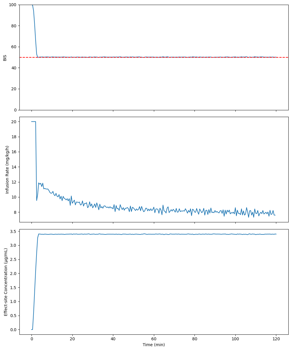
Initial BIS: 100.00
Final BIS: 50.04
Mean infusion rate: 8.85 mg/kg/h
Final effect-site concentration: 3.40 µg/mL