Dynamic Programming#
Unlike the methods we’ve discussed so far, dynamic programming takes a step back and considers an entire family of related problems rather than a single optimization problem. This approach, while seemingly more complex at first glance, can often lead to efficient solutions.
Dynamic programming leverage the solution structure underlying many control problems that allows for a decomposition it into smaller, more manageable subproblems. Each subproblem is itself an optimization problem, embedded within the larger whole. This recursive structure is the foundation upon which dynamic programming constructs its solutions.
To ground our discussion, let us return to the domain of discrete-time optimal control problems (DOCPs). These problems frequently arise from the discretization of continuous-time optimal control problems. While the focus here will be on deterministic problems, it is worth noting that these concepts extend naturally to stochastic problems by taking the expectation over the random quantities.
Consider a typical DOCP of Bolza type:
Rather than considering only the total cost from the initial time to the final time, dynamic programming introduces the concept of cost from an arbitrary point in time to the end. This leads to the definition of the “cost-to-go” or “value function” \(J_k(\mathbf{x}_k)\):
This function represents the total cost incurred from stage \(k\) onwards to the end of the time horizon, given that the system is initialized in state \(\mathbf{x}_k\) at stage \(k\). Suppose the problem has been solved from stage \(k+1\) to the end, yielding the optimal cost-to-go \(J_{k+1}^\star(\mathbf{x}_{k+1})\) for any state \(\mathbf{x}_{k+1}\) at stage \(k+1\). The question then becomes: how does this information inform the decision at stage \(k\)?
Given knowledge of the optimal behavior from \(k+1\) onwards, the task reduces to determining the optimal action \(\mathbf{u}_k\) at stage \(k\). This control should minimize the sum of the immediate cost \(c_k(\mathbf{x}_k, \mathbf{u}_k)\) and the optimal future cost \(J_{k+1}^\star(\mathbf{x}_{k+1})\), where \(\mathbf{x}_{k+1}\) is the resulting state after applying action \(\mathbf{u}_k\). Mathematically, this is expressed as:
This equation is known as Bellman’s equation, named after Richard Bellman, who formulated the principle of optimality:
An optimal policy has the property that whatever the previous state and decision, the remaining decisions must constitute an optimal policy with regard to the state resulting from the previous decision.
In other words, any sub-path of an optimal path, from any intermediate point to the end, must itself be optimal. This principle is the basis for the backward induction procedure which computes the optimal value function and provides closed-loop control capabilities without having to use an explicit NLP solver.
Dynamic programming can handle nonlinear systems and non-quadratic cost functions naturally. It provides a global optimal solution, when one exists, and can incorporate state and control constraints with relative ease. However, as the dimension of the state space increases, this approach suffers from what Bellman termed the “curse of dimensionality.” The computational complexity and memory requirements grow exponentially with the state dimension, rendering direct application of dynamic programming intractable for high-dimensional problems.
Fortunately, learning-based methods offer efficient tools to combat the curse of dimensionality on two fronts: by using function approximation (e.g., neural networks) to avoid explicit discretization, and by leveraging randomization through Monte Carlo methods inherent in the learning paradigm. Most of this course is dedicated to those ideas.
Backward Recursion#
The principle of optimality provides a methodology for solving optimal control problems. Beginning at the final time horizon and working backwards, at each stage the local optimization problem given by Bellman’s equation is solved. This process, termed backward recursion or backward induction, constructs the optimal value function stage by stage.
Algorithm 3 (Backward Recursion for Dynamic Programming)
Input: Terminal cost function \(c_\mathrm{T}(\cdot)\), stage cost functions \(c_t(\cdot, \cdot)\), system dynamics \(f_t(\cdot, \cdot)\), time horizon \(\mathrm{T}\)
Output: Optimal value functions \(J_t^\star(\cdot)\) and optimal control policies \(\mu_t^\star(\cdot)\) for \(t = 1, \ldots, T\)
Initialize \(J_T^\star(\mathbf{x}) = c_\mathrm{T}(\mathbf{x})\) for all \(\mathbf{x}\) in the state space
For \(t = T-1, T-2, \ldots, 1\):
For each state \(\mathbf{x}\) in the state space:
Compute \(J_t^\star(\mathbf{x}) = \min_{\mathbf{u}} \left[ c_t(\mathbf{x}, \mathbf{u}) + J_{t+1}^\star(f_t(\mathbf{x}, \mathbf{u})) \right]\)
Compute \(\mu_t^\star(\mathbf{x}) = \arg\min_{\mathbf{u}} \left[ c_t(\mathbf{x}, \mathbf{u}) + J_{t+1}^\star(f_t(\mathbf{x}, \mathbf{u})) \right]\)
End For
End For
Return \(J_t^\star(\cdot)\), \(\mu_t^\star(\cdot)\) for \(t = 1, \ldots, T\)
Upon completion of this backward pass, we now have access to the optimal control to take at any stage and in any state. Furthermore, we can simulate optimal trajectories from any initial state and applying the optimal policy at each stage to generate the optimal trajectory.
Theorem 2 (Backward induction solves deterministic Bolza DOCP)
Setting. Let \(\mathbf{x}_{t+1}=\mathbf{f}_t(\mathbf{x}_t,\mathbf{u}_t)\) for \(t=1,\dots,T-1\), with admissible action sets \(\mathcal{U}_t(\mathbf{x})\neq\varnothing\). Let stage costs \(c_t(\mathbf{x},\mathbf{u})\) and terminal cost \(c_\mathrm{T}(\mathbf{x})\) be real-valued and bounded below. Assume for every \((t,\mathbf{x})\) the one-step problem
admits a minimizer (e.g., compact \(\mathcal{U}_t(\mathbf{x})\) and continuity suffice).
Define \(J_T^\star(\mathbf{x}) \equiv c_\mathrm{T}(\mathbf{x})\) and for \(t=T-1,\dots,1\)
and select any minimizer \(\boldsymbol{\mu}_t^\star(\mathbf{x})\in\arg\min(\cdot)\).
Claim. For every initial state \(\mathbf{x}_1\), the control sequence \(\boldsymbol{\mu}_1^\star(\mathbf{x}_1),\dots,\boldsymbol{\mu}_{T-1}^\star(\mathbf{x}_{T-1})\) generated by these selectors is optimal for the Bolza problem, and \(J_1^\star(\mathbf{x}_1)\) equals the optimal cost. Moreover, \(J_t^\star(\cdot)\) is the optimal cost-to-go from stage \(t\) for every state, i.e., backward induction recovers the entire value function.
Proof. We give a direct proof by backward induction. The general idea is that any feasible sequence can be improved by replacing its tail with an optimal continuation, so optimal solutions can be built stage by stage. This is sometimes called a “cut-and-paste” argument.
Step 1 (verification of the recursion at a fixed stage).
Fix \(t\in\{1,\dots,T-1\}\) and \(\mathbf{x}\in\mathbb{X}\). Consider any admissible control sequence \(\mathbf{u}_t,\dots,\mathbf{u}_{T-1}\) starting from \(\mathbf{x}_t=\mathbf{x}\) and define the induced states \(\mathbf{x}_{k+1}=\mathbf{f}_k(\mathbf{x}_k,\mathbf{u}_k)\). Its total cost from \(t\) is
By definition of \(J_{t+1}^\star\), the tail cost satisfies
Hence the total cost is bounded below by
Taking the minimum over \(\mathbf{u}_t\in\mathcal{U}_t(\mathbf{x})\) yields
Step 2 (existence of an optimal prefix at stage \(t\)).
By assumption, there exists \(\boldsymbol{\mu}_t^\star(\mathbf{x})\) attaining the minimum in the definition of \(J_t^\star(\mathbf{x})\). If we now paste to \(\boldsymbol{\mu}_t^\star(\mathbf{x})\) an optimal tail policy from \(t+1\) (whose existence we will establish inductively), the resulting sequence attains cost exactly
which matches the lower bound \((\ast)\); hence it is optimal from \(t\).
Step 3 (backward induction over time).
Base case \(t=T\). The statement holds because \(J_T^\star(\mathbf{x})=c_\mathrm{T}(\mathbf{x})\) and there is no control to choose.
Inductive step. Assume the tail statement holds for \(t+1\): from any state \(\mathbf{x}_{t+1}\) there exists an optimal control sequence realizing \(J_{t+1}^\star(\mathbf{x}_{t+1})\). Then by Steps 1–2, selecting \(\boldsymbol{\mu}_t^\star(\mathbf{x}_t)\) at stage \(t\) and concatenating the optimal tail from \(t+1\) yields an optimal sequence from \(t\) with value \(J_t^\star(\mathbf{x}_t)\).
By backward induction, the claim holds for all \(t\), in particular for \(t=1\) and any initial \(\mathbf{x}_1\). Therefore the backward recursion both certifies optimality (verification) and constructs an optimal policy (synthesis), while recovering the full family \(\{J_t^\star\}_{t=1}^T\).
Remark 1 (No “big NLP” required)
The Bolza DOCP over the whole horizon couples all controls through the dynamics and is typically posed as a single large nonlinear program. The proof shows you can solve \(T-1\) sequences of one-step problems instead: at each \((t,\mathbf{x})\) minimize
In finite state–action spaces this becomes pure table lookup and argmin. In continuous spaces you still solve local one-step minimizations, but you avoid a monolithic horizon-coupled NLP.
Remark 2 (Graph interpretation (optional intuition))
Unroll time to form a DAG whose nodes are \((t,\mathbf{x})\) and whose edges correspond to feasible controls with edge weight \(c_t(\mathbf{x},\mathbf{u})\). The terminal node cost is \(c_\mathrm{T}(\cdot)\). The Bolza problem is a shortest-path problem on this DAG. The equation
is exactly the dynamic programming recursion for shortest paths on acyclic graphs, hence backward induction is optimal.
Example: Optimal Harvest in Resource Management#
Dynamic programming is often used in resource management and conservation biology to devise policies to be implemented by decision makers and stakeholders : for eg. in fishereries, or timber harvesting. Per [9], we consider a population of a particular species, whose abundance we denote by \(x_t\), where \(t\) represents discrete time steps. Our objective is to maximize the cumulative harvest over a finite time horizon, while also considering the long-term sustainability of the population. This optimization problem can be formulated as:
Here, \(F(\cdot)\) represents the immediate reward function associated with harvesting, \(h_t\) is the harvest rate at time \(t\), and \(F_\mathrm{T}(\cdot)\) denotes a terminal value function that could potentially assign value to the final population state. In this particular problem, we assign no terminal value to the final population state, setting \(F_\mathrm{T}(x_{t_f}) = 0\) and allowing us to focus solely on the cumulative harvest over the time horizon.
In our model population model, the abundance of a specicy \(x\) ranges from 1 to 100 individuals. The decision variable is the harvest rate \(h\), which can take values from the set \(D = \{0, 0.1, 0.2, 0.3, 0.4, 0.5\}\). The population dynamics are governed by a modified logistic growth model:
where the \(0.3\) represents the growth rate and \(125\) is the carrying capacity (the maximum population size given the available resources). The logistic growth model returns continuous values; however our DP formulation uses a discrete state space. Therefore, we also round the the outcomes to the nearest integer.
Applying the principle of optimality, we can express the optimal value function \(J^\star(x_t,t)\) recursively:
with the boundary condition \(J^*(x_{t_f}) = 0\).
It’s worth noting that while this example uses a relatively simple model, the same principles can be applied to more complex scenarios involving stochasticity, multiple species interactions, or spatial heterogeneity.
Show code cell source
import numpy as np

# Parameters
r_max = 0.3
K = 125
T = 20  # Number of time steps
N_max = 100  # Maximum population size to consider
h_max = 0.5  # Maximum harvest rate
h_step = 0.1  # Step size for harvest rate

# Create state and decision spaces
N_space = np.arange(1, N_max + 1)
h_space = np.arange(0, h_max + h_step, h_step)

# Initialize value function and policy
V = np.zeros((T + 1, len(N_space)))
policy = np.zeros((T, len(N_space)))

# Terminal value function (F_T)
def terminal_value(N):
    return 0

# State return function (F)
def state_return(N, h):
    return N * h

# State dynamics function
def state_dynamics(N, h):
    return N + r_max * N * (1 - N / K) - N * h

# Backward iteration
for t in range(T - 1, -1, -1):
    for i, N in enumerate(N_space):
        max_value = float('-inf')
        best_h = 0

        for h in h_space:
            if h > 1:  # Ensure harvest rate doesn't exceed 100%
                continue

            next_N = state_dynamics(N, h)
            if next_N < 1:  # Ensure population doesn't go extinct
                continue

            next_N_index = np.searchsorted(N_space, next_N)
            if next_N_index == len(N_space):
                next_N_index -= 1

            value = state_return(N, h) + V[t + 1, next_N_index]

            if value > max_value:
                max_value = value
                best_h = h

        V[t, i] = max_value
        policy[t, i] = best_h

# Function to simulate the optimal policy with conversion to Python floats
def simulate_optimal_policy(initial_N, T):
    trajectory = [float(initial_N)]  # Ensure first value is a Python float
    harvests = []

    for t in range(T):
        N = trajectory[-1]
        N_index = np.searchsorted(N_space, N)
        if N_index == len(N_space):
            N_index -= 1

        h = policy[t, N_index]
        harvests.append(float(N * h))  # Ensure harvest is a Python float

        next_N = state_dynamics(N, h)
        trajectory.append(float(next_N))  # Ensure next population value is a Python float

    return trajectory, harvests

# Example usage
initial_N = 50
trajectory, harvests = simulate_optimal_policy(initial_N, T)

print("Optimal policy:")
print(policy)
print("\nPopulation trajectory:", trajectory)
print("Harvests:", harvests)
print("Total harvest:", sum(harvests))
Optimal policy:
[[0.2 0.2 0.2 ... 0.4 0.4 0.5]
 [0.2 0.2 0.2 ... 0.4 0.4 0.5]
 [0.2 0.2 0.2 ... 0.4 0.4 0.4]
 ...
 [0.2 0.2 0.2 ... 0.5 0.5 0.5]
 [0.2 0.5 0.5 ... 0.5 0.5 0.5]
 [0.2 0.5 0.5 ... 0.5 0.5 0.5]]

Population trajectory: [50.0, 54.0, 63.2016, 53.614938617856, 62.80047226002128, 65.89520835342945, 62.063500827311884, 65.23169346891407, 61.5424456170318, 64.7610004703774, 61.171531280797, 64.42514256278633, 60.90621923290014, 52.003257133909514, 61.11382126799714, 64.37282756165249, 60.86484408994034, 39.80100508132969, 28.038916051902078, 20.544298889444192, 15.422475391094192]
Harvests: [5.0, 0.0, 18.960480000000004, 0.0, 6.280047226002129, 13.17904167068589, 6.206350082731189, 13.046338693782815, 6.15424456170318, 12.95220009407548, 6.1171531280797, 12.885028512557268, 18.271865769870047, 0.0, 6.111382126799715, 12.874565512330499, 30.43242204497017, 19.900502540664846, 14.019458025951039, 10.272149444722096]
Total harvest: 212.66322943492605
Handling Continuous Spaces with Interpolation#
In many real-world problems, such as our resource management example, the state space is inherently continuous. Dynamic programming, however, is usually defined on discrete state spaces. To reconcile this, we approximate the value function on a finite grid of points and use interpolation to estimate its value elsewhere.
In our earlier example, we acted as if population sizes could only be whole numbers: 1 fish, 2 fish, 3 fish. But real measurements don’t fit neatly. What do you do with a survey that reports 42.7 fish? Our reflex in the code example was to round to the nearest integer, effectively saying “let’s just call it 43.” This corresponds to nearest-neighbor interpolation, also known as discretization. It’s the zeroth-order case: you assume the value between grid points is constant and equal to the closest one. In practice, this amounts to overlaying a grid on the continuous landscape and forcing yourself to stand at the intersections. In our demo code, this step was carried out with numpy.searchsorted.
While easy to implement, nearest-neighbor interpolation can introduce artifacts:
Decisions may change abruptly, even if the state only shifts slightly.
Precision is lost, especially in regimes where small variations matter.
The curse of dimensionality forces an impractically fine grid if many state variables are added.
To address these issues, we can use higher-order interpolation. Instead of taking the nearest neighbor, we estimate the value at off-grid points by leveraging multiple nearby values.
Backward Recursion with Interpolation#
Suppose we have computed \(J_{k+1}^\star(\mathbf{x})\) only at grid points \(\mathbf{x} \in \mathcal{X}_\text{grid}\). To evaluate Bellman’s equation at an arbitrary \(\mathbf{x}_{k+1}\), we interpolate. Formally, let \(I_{k+1}(\mathbf{x})\) be the interpolation operator that extends the value function from \(\mathcal{X}_\text{grid}\) to the continuous space. Then:
For instance, in one dimension, linear interpolation gives:
where \(x_l\) and \(x_u\) are the nearest grid points bracketing \(x\). Linear interpolation is often sufficient, but higher-order methods (cubic splines, radial basis functions) can yield smoother and more accurate estimates. The choice of interpolation scheme and grid layout both affect accuracy and efficiency. A finer grid improves resolution but increases computational cost, motivating strategies like adaptive grid refinement or replacing interpolation altogether with parametric function approximation which we are going to see later in this book.
In higher-dimensional spaces, naive interpolation becomes prohibitively expensive due to the curse of dimensionality. Several approaches such as tensorized multilinear interpolation, radial basis functions, and machine learning models address this challenge by extending a common principle: they approximate the value function at unobserved points using information from a finite set of evaluations. However, as dimensionality continues to grow, even tensor methods face scalability limits, which is why flexible parametric models like neural networks have become essential tools for high-dimensional function approximation.
Algorithm 4 (Backward Recursion with Interpolation)
Input:
Terminal cost \(c_\mathrm{T}(\cdot)\)
Stage costs \(c_t(\cdot,\cdot)\)
Dynamics \(f_t(\cdot,\cdot)\)
Time horizon \(T\)
State grid \(\mathcal{X}_\text{grid}\)
Action set \(\mathcal{U}\)
Interpolation method \(\mathcal{I}(\cdot)\) (e.g., linear, cubic spline, RBF, neural network)
Output: Value functions \(J_t^\star(\cdot)\) and policies \(\mu_t^\star(\cdot)\) for all \(t\)
Initialize terminal values:
Compute \(J_T^\star(\mathbf{x}) = c_\mathrm{T}(\mathbf{x})\) for all \(\mathbf{x} \in \mathcal{X}_\text{grid}\)
Fit interpolator: \(I_T \leftarrow \mathcal{I}(\{\mathbf{x}, J_T^\star(\mathbf{x})\}_{\mathbf{x} \in \mathcal{X}_\text{grid}})\)
Backward recursion:
For \(t = T-1, T-2, \dots, 0\):a. Bellman update at grid points:
For each \(\mathbf{x} \in \mathcal{X}_\text{grid}\):For each \(\mathbf{u} \in \mathcal{U}\):
Compute next state: \(\mathbf{x}_\text{next} = f_t(\mathbf{x}, \mathbf{u})\)
Interpolate future cost: \(\hat{J}_{t+1}(\mathbf{x}_\text{next}) = I_{t+1}(\mathbf{x}_\text{next})\)
Compute total cost: \(J_t(\mathbf{x}, \mathbf{u}) = c_t(\mathbf{x}, \mathbf{u}) + \hat{J}_{t+1}(\mathbf{x}_\text{next})\)
Minimize over actions: \(J_t^\star(\mathbf{x}) = \min_{\mathbf{u} \in \mathcal{U}} J_t(\mathbf{x}, \mathbf{u})\)
Store optimal action: \(\mu_t^\star(\mathbf{x}) = \arg\min_{\mathbf{u} \in \mathcal{U}} J_t(\mathbf{x}, \mathbf{u})\)
b. Fit interpolator for current stage:
\(I_t \leftarrow \mathcal{I}(\{\mathbf{x}, J_t^\star(\mathbf{x})\}_{\mathbf{x} \in \mathcal{X}_\text{grid}})\)Return: Interpolated value functions \(\{I_t\}_{t=0}^T\) and policies \(\{\mu_t^\star\}_{t=0}^{T-1}\)
Example: Optimal Harvest with Linear Interpolation#
Here is a demonstration of the backward recursion procedure using linear interpolation.
Show code cell source
import numpy as np

# Parameters
r_max = 0.3
K = 125
T = 20  # Number of time steps
N_max = 100  # Maximum population size to consider
h_max = 0.5  # Maximum harvest rate
h_step = 0.1  # Step size for harvest rate

# Create state and decision spaces
N_space = np.arange(1, N_max + 1)
h_space = np.arange(0, h_max + h_step, h_step)

# Initialize value function and policy
V = np.zeros((T + 1, len(N_space)))
policy = np.zeros((T, len(N_space)))

# Terminal value function (F_T)
def terminal_value(N):
    return 0

# State return function (F)
def state_return(N, h):
    return N * h

# State dynamics function
def state_dynamics(N, h):
    return N + r_max * N * (1 - N / K) - N * h

# Function to linearly interpolate between grid points in N_space
def interpolate_value_function(V, N_space, next_N, t):
    if next_N <= N_space[0]:
        return V[t, 0]  # Below or at minimum population, return minimum value
    if next_N >= N_space[-1]:
        return V[t, -1]  # Above or at maximum population, return maximum value

    # Find indices to interpolate between
    lower_idx = np.searchsorted(N_space, next_N) - 1
    upper_idx = lower_idx + 1

    # Linear interpolation
    N_lower = N_space[lower_idx]
    N_upper = N_space[upper_idx]
    weight = (next_N - N_lower) / (N_upper - N_lower)
    return (1 - weight) * V[t, lower_idx] + weight * V[t, upper_idx]

# Backward iteration with interpolation
for t in range(T - 1, -1, -1):
    for i, N in enumerate(N_space):
        max_value = float('-inf')
        best_h = 0

        for h in h_space:
            if h > 1:  # Ensure harvest rate doesn't exceed 100%
                continue

            next_N = state_dynamics(N, h)
            if next_N < 1:  # Ensure population doesn't go extinct
                continue

            # Interpolate value for next_N
            value = state_return(N, h) + interpolate_value_function(V, N_space, next_N, t + 1)

            if value > max_value:
                max_value = value
                best_h = h

        V[t, i] = max_value
        policy[t, i] = best_h

# Function to simulate the optimal policy using interpolation
def simulate_optimal_policy(initial_N, T):
    trajectory = [initial_N]
    harvests = []

    for t in range(T):
        N = trajectory[-1]

        # Interpolate optimal harvest rate
        if N <= N_space[0]:
            h = policy[t, 0]
        elif N >= N_space[-1]:
            h = policy[t, -1]
        else:
            lower_idx = np.searchsorted(N_space, N) - 1
            upper_idx = lower_idx + 1
            weight = (N - N_space[lower_idx]) / (N_space[upper_idx] - N_space[lower_idx])
            h = (1 - weight) * policy[t, lower_idx] + weight * policy[t, upper_idx]

        harvests.append(float(N * h))  # Ensure harvest is a Python float
        next_N = state_dynamics(N, h)
        trajectory.append(float(next_N))  # Ensure next population value is a Python float

    return trajectory, harvests

# Example usage
initial_N = 50
trajectory, harvests = simulate_optimal_policy(initial_N, T)

print("Optimal policy:")
print(policy)
print("\nPopulation trajectory:", trajectory)
print("Harvests:", harvests)
print("Total harvest:", sum(harvests))
Optimal policy:
[[0.  0.  0.  ... 0.4 0.4 0.4]
 [0.  0.  0.  ... 0.4 0.4 0.4]
 [0.  0.  0.  ... 0.4 0.4 0.4]
 ...
 [0.  0.  0.3 ... 0.5 0.5 0.5]
 [0.2 0.5 0.5 ... 0.5 0.5 0.5]
 [0.2 0.5 0.5 ... 0.5 0.5 0.5]]

Population trajectory: [50, 59.0, 62.445600000000006, 62.793456961535966, 60.906514028106535, 64.1847685511936, 60.71600257278426, 64.0117639631371, 60.5789261378371, 63.88717626457206, 60.48012279248407, 63.79731874379539, 60.40881570882111, 63.73243881376377, 60.3573056779798, 63.685556376683536, 60.32007179593332, 39.523630889226936, 27.8698229545787, 20.431713488016012, 15.34347899187751]
Harvests: [0.0, 5.9, 9.027135936000038, 11.26173625265758, 6.0906514028106535, 12.83695371023872, 6.071600257278426, 12.80235279262742, 6.057892613783711, 12.777435252914414, 6.0480122792484075, 12.759463748759078, 6.040881570882111, 12.746487762752755, 6.03573056779798, 12.737111275336709, 30.16003589796666, 19.761815444613468, 13.93491147728935, 10.215856744008006]
Total harvest: 213.2660649869655
Due to pedagogical considerations, this example is using our own implementation of the linear interpolation procedure. However, a more general and practical approach would be to use a built-in interpolation procedure in Numpy. Because our state space has a single dimension, we can simply use scipy.interpolate.interp1d which offers various interpolation methods through its kind argument, which can take values in ‘linear’, ‘nearest’, ‘nearest-up’, ‘zero’, ‘slinear’, ‘quadratic’, ‘cubic’, ‘previous’, or ‘next’. ‘zero’, ‘slinear’, ‘quadratic’ and ‘cubic’.
Here’s a more general implementation which here uses cubic interpolation through the scipy.interpolate.interp1d function:
Show code cell source
import numpy as np
from scipy.interpolate import interp1d

# Parameters
r_max = 0.3
K = 125
T = 20  # Number of time steps
N_max = 100  # Maximum population size to consider
h_max = 0.5  # Maximum harvest rate
h_step = 0.1  # Step size for harvest rate

# Create state and decision spaces
N_space = np.arange(1, N_max + 1)
h_space = np.arange(0, h_max + h_step, h_step)

# Initialize value function and policy
V = np.zeros((T + 1, len(N_space)))
policy = np.zeros((T, len(N_space)))

# Terminal value function (F_T)
def terminal_value(N):
    return 0

# State return function (F)
def state_return(N, h):
    return N * h

# State dynamics function
def state_dynamics(N, h):
    return N + r_max * N * (1 - N / K) - N * h

# Function to create interpolation function for a given time step
def create_interpolator(V_t, N_space):
    return interp1d(N_space, V_t, kind='cubic', bounds_error=False, fill_value=(V_t[0], V_t[-1]))

# Backward iteration with interpolation
for t in range(T - 1, -1, -1):
    interpolator = create_interpolator(V[t+1], N_space)

    for i, N in enumerate(N_space):
        max_value = float('-inf')
        best_h = 0

        for h in h_space:
            if h > 1:  # Ensure harvest rate doesn't exceed 100%
                continue

            next_N = state_dynamics(N, h)
            if next_N < 1:  # Ensure population doesn't go extinct
                continue

            # Use interpolation to get the value for next_N
            value = state_return(N, h) + interpolator(next_N)

            if value > max_value:
                max_value = value
                best_h = h

        V[t, i] = max_value
        policy[t, i] = best_h

# Function to simulate the optimal policy using interpolation
def simulate_optimal_policy(initial_N, T):
    trajectory = [initial_N]
    harvests = []

    for t in range(T):
        N = trajectory[-1]

        # Create interpolator for the policy at time t
        policy_interpolator = interp1d(N_space, policy[t], kind='cubic', bounds_error=False, fill_value=(policy[t][0], policy[t][-1]))

        h = policy_interpolator(N)
        harvests.append(float(N * h))  # Ensure harvest is a Python float

        next_N = state_dynamics(N, h)
        trajectory.append(float(next_N))  # Ensure next population value is a Python float

    return trajectory, harvests

# Example usage
initial_N = 50
trajectory, harvests = simulate_optimal_policy(initial_N, T)

print("Optimal policy (first few rows):")
print(policy[:5])
print("\nPopulation trajectory:", trajectory)
print("Harvests:", harvests)
print("Total harvest:", sum(harvests))
Optimal policy (first few rows):
[[0.  0.  0.  0.  0.  0.  0.  0.  0.  0.  0.  0.  0.  0.  0.  0.  0.  0.
  0.  0.  0.  0.  0.  0.  0.  0.  0.  0.  0.  0.  0.  0.  0.  0.  0.  0.
  0.  0.  0.  0.  0.  0.  0.  0.  0.  0.  0.  0.  0.  0.  0.  0.  0.  0.
  0.  0.  0.1 0.1 0.1 0.1 0.1 0.1 0.2 0.2 0.2 0.2 0.2 0.2 0.2 0.2 0.2 0.3
  0.3 0.3 0.3 0.3 0.3 0.3 0.3 0.3 0.3 0.3 0.3 0.4 0.4 0.4 0.4 0.4 0.4 0.4
  0.4 0.4 0.4 0.4 0.4 0.4 0.4 0.4 0.4 0.4]
 [0.  0.  0.  0.  0.  0.  0.  0.  0.  0.  0.  0.  0.  0.  0.  0.  0.  0.
  0.  0.  0.  0.  0.  0.  0.  0.  0.  0.  0.  0.  0.  0.  0.  0.  0.  0.
  0.  0.  0.  0.  0.  0.  0.  0.  0.  0.  0.  0.  0.  0.  0.  0.  0.  0.
  0.  0.  0.1 0.1 0.1 0.1 0.1 0.1 0.1 0.2 0.2 0.2 0.2 0.2 0.2 0.2 0.2 0.3
  0.3 0.3 0.3 0.3 0.3 0.3 0.3 0.3 0.3 0.3 0.4 0.4 0.4 0.4 0.4 0.4 0.4 0.4
  0.4 0.4 0.4 0.4 0.4 0.4 0.4 0.4 0.4 0.4]
 [0.  0.  0.  0.  0.  0.  0.  0.  0.  0.  0.  0.  0.  0.  0.  0.  0.  0.
  0.  0.  0.  0.  0.  0.  0.  0.  0.  0.  0.  0.  0.  0.  0.  0.  0.  0.
  0.  0.  0.  0.  0.  0.  0.  0.  0.  0.  0.  0.  0.  0.  0.  0.  0.  0.
  0.  0.  0.1 0.1 0.1 0.1 0.1 0.1 0.2 0.2 0.2 0.2 0.2 0.2 0.2 0.2 0.2 0.3
  0.3 0.3 0.3 0.3 0.3 0.3 0.3 0.3 0.3 0.3 0.3 0.4 0.4 0.4 0.4 0.4 0.4 0.4
  0.4 0.4 0.4 0.4 0.4 0.4 0.4 0.4 0.4 0.4]]

Population trajectory: [50, 59.0, 62.445600000000006, 62.855816819468515, 66.38501069094303, 62.46338144008508, 66.19082983826176, 62.307060290079974, 65.86630883298251, 62.0275406161329, 65.08602250342238, 61.40579635061663, 65.16431296091169, 61.453283417050585, 65.25607512917725, 61.51516182245858, 65.3615391678991, 42.035857104726354, 29.387853805711547, 21.437532761435143, 16.047063462998082]
Harvests: [3.3073317494565994e-20, 5.8999999999999995, 8.96477607806749, 5.84550227506383, 13.260405311492967, 5.647548383617885, 13.22607620843378, 5.815662115341462, 13.186571332467969, 6.31598238982395, 13.039176123074048, 5.613609913801768, 13.068992991332264, 5.569578810421298, 13.097683026436256, 5.526294879593217, 32.68102988779014, 21.017928552363177, 14.693926902855772, 10.718766380713353]
Total harvest: 213.18951156269063
Stochastic Dynamic Programming and Markov Decision Processes#
While our previous discussion centered on deterministic systems, many real-world problems involve uncertainty. Stochastic Dynamic Programming (SDP) extends our framework to handle stochasticity in both the objective function and system dynamics. This extension naturally leads us to consider more general policy classes and to formalize when simpler policies suffice.
Decision Rules and Policies#
Before diving into stochastic systems, we need to establish terminology for the different types of strategies a decision maker might employ. In the deterministic setting, we implicitly used feedback controllers of the form \(u(\mathbf{x}, t)\). In the stochastic setting, we must be more precise about what information policies can use and how they select actions.
A decision rule is a prescription for action selection in each state at a specified decision epoch. These rules can vary in their complexity based on two main criteria:
Dependence on history: Markovian or History-dependent
Action selection method: Deterministic or Randomized
Markovian decision rules depend only on the current state, while history-dependent rules consider the entire sequence of past states and actions. Formally, a history \(h_t\) at time \(t\) is:
The set of all possible histories at time \(t\), denoted \(H_t\), grows exponentially with \(t\):
\(H_1 = \mathcal{S}\) (just the initial state)
\(H_2 = \mathcal{S} \times \mathcal{A} \times \mathcal{S}\)
\(H_t = \mathcal{S} \times (\mathcal{A} \times \mathcal{S})^{t-1}\)
Deterministic rules select an action with certainty, while randomized rules specify a probability distribution over the action space.
These classifications lead to four types of decision rules:
Markovian Deterministic (MD): \(\pi_t: \mathcal{S} \rightarrow \mathcal{A}_s\)
Markovian Randomized (MR): \(\pi_t: \mathcal{S} \rightarrow \mathcal{P}(\mathcal{A}_s)\)
History-dependent Deterministic (HD): \(\pi_t: H_t \rightarrow \mathcal{A}_s\)
History-dependent Randomized (HR): \(\pi_t: H_t \rightarrow \mathcal{P}(\mathcal{A}_s)\)
where \(\mathcal{P}(\mathcal{A}_s)\) denotes the set of probability distributions over \(\mathcal{A}_s\).
A policy \(\boldsymbol{\pi}\) is a sequence of decision rules, one for each decision epoch:
The set of all policies of class \(K\) (where \(K \in \{HR, HD, MR, MD\}\)) is denoted as \(\Pi^K\). These policy classes form a hierarchy:
The largest set \(\Pi^{HR}\) contains all possible policies. We ask: under what conditions can we restrict attention to the much simpler set \(\Pi^{MD}\) without loss of optimality?
Notation: rules vs. policies
Decision rule (kernel). A map from information to action distributions:
Markov, deterministic: \(\pi_t:\mathcal{S}\to\mathcal{A}_s\)
Markov, randomized: \(\pi_t(\cdot\mid s)\in\Delta(\mathcal{A}_s)\)
History-dependent: \(\pi_t(\cdot\mid h_t)\in\Delta(\mathcal{A}_{s_t})\)
Policy (sequence). \(\boldsymbol{\pi}=(\pi_1,\pi_2,\ldots)\).
Stationary policy. \(\boldsymbol{\pi}=\mathrm{const}(\pi)\) with \(\pi_t\equiv\pi \ \forall t\).
By convention, we identify \(\pi\) with its stationary policy \(\mathrm{const}(\pi)\) when no confusion arises.
Stochastic System Dynamics#
In the stochastic setting, our system evolution takes the form:
Here, \(\mathbf{w}_t\) represents a random disturbance or noise term at time \(t\) due to the inherent uncertainty in the system’s behavior. The stage cost function may also incorporate stochastic influences:
In this context, our objective shifts from minimizing a deterministic cost to minimizing the expected total cost:
where the expectation is taken over the distributions of the random variables \(\mathbf{w}_t\). The principle of optimality still holds in the stochastic case, but Bellman’s optimality equation now involves an expectation:
In practice, this expectation is often computed by discretizing the distribution of \(\mathbf{w}_k\) when the set of possible disturbances is very large or even continuous. Let’s say we approximate the distribution with \(K\) discrete values \(\mathbf{w}_k^i\), each occurring with probability \(p_k^i\). Then our Bellman equation becomes:
Optimality Equations in the Stochastic Setting#
When dealing with stochastic systems, a central question arises: what information should our control policy use? In the most general case, a policy might use the entire history of observations and actions. However, as we’ll see, the Markovian structure of our problems allows for dramatic simplifications.
Let \(h_t = (s_1, a_1, s_2, a_2, \ldots, s_{t-1}, a_{t-1}, s_t)\) denote the complete history up to time \(t\). In the stochastic setting, the history-based optimality equations become:
where we now explicitly use the transition probabilities \(p_t(j|s_t,a)\) rather than a deterministic dynamics function.
Theorem 3 (Principle of optimality for stochastic systems)
Let \(u_t^*\) be the optimal expected return from epoch \(t\) onward. Then:
a. \(u_t^*\) satisfies the optimality equations:
with boundary condition \(u_N^*(h_N) = r_N(s_N)\).
b. Any policy \(\pi^*\) that selects actions attaining the supremum (or maximum) in the above equation at each history is optimal.
Intuition: This formalizes Bellman’s principle of optimality: “An optimal policy has the property that whatever the initial state and initial decision are, the remaining decisions must constitute an optimal policy with regard to the state resulting from the first decision.” The recursive structure means that optimal local decisions (choosing the best action at each step) lead to global optimality, even with uncertainty captured by the transition probabilities.
A remarkable simplification occurs when we examine these history-based equations more closely. The Markov property of our system dynamics and rewards means that the optimal return actually depends on the history only through the current state:
Proposition 2 (State sufficiency for stochastic MDPs)
In finite-horizon stochastic MDPs with Markovian dynamics and rewards, the optimal return \(u_t^*(h_t)\) depends on the history only through the current state \(s_t\). Thus we can write \(u_t^*(h_t) = v_t^*(s_t)\) for some function \(v_t^*\) that depends only on state and time.
Proof. Following Puterman [34] Theorem 4.4.2. We proceed by backward induction.
Base case: At the terminal time \(N\), we have \(u_N^*(h_N) = r_N(s_N)\) by the boundary condition. Since the terminal reward depends only on the final state \(s_N\) and not on how we arrived there, \(u_N^*(h_N) = u_N^*(s_N)\).
Inductive step: Assume \(u_{t+1}^*(h_{t+1})\) depends on \(h_{t+1}\) only through \(s_{t+1}\) for all \(t+1, \ldots, N\). Then from the optimality equation:
By the induction hypothesis, \(u_{t+1}^*(h_t, a, j)\) depends only on the next state \(j\), so:
Since the expression in brackets depends on \(h_t\) only through the current state \(s_t\) (the rewards and transition probabilities are Markovian), we conclude that \(u_t^*(h_t) = u_t^*(s_t)\).
Intuition: The Markov property means that the current state contains all information needed to predict future evolution. The past provides no additional value for decision-making. This powerful result allows us to work with value functions \(v_t^*(s)\) indexed only by state and time, dramatically simplifying both theory and computation.
This state-sufficiency result, combined with the fact that randomization never helps when maximizing expected returns, leads to a dramatic simplification of the policy space:
Theorem 4 (Policy reduction for stochastic MDPs)
For finite-horizon stochastic MDPs with finite state and action sets:
That is, there exists an optimal policy that is both deterministic and Markovian.
Proof. Sketch following Puterman [34] Lemma 4.3.1 and Theorem 4.4.2. First, Lemma 4.3.1 shows that for any function \(w\) and any distribution \(q\) over actions, \(\sup_a w(a) \ge \sum_a q(a) w(a)\). Thus randomization cannot improve the expected value over choosing a single maximizing action. Second, by state sufficiency (Proposition stoch-state-suff and Puterman [34] Thm. 4.4.2(a)), the optimal return depends on the history only through \((s_t,t)\). Therefore, selecting at each \((s_t,t)\) an action that attains the maximum yields a deterministic Markov decision rule which is optimal whenever the maximum is attained. If only a supremum exists, \(\varepsilon\)-optimal selectors exist by choosing actions within \(\varepsilon\) of the supremum (see Puterman [34] Thm. 4.3.4).
Intuition: Even in stochastic systems, randomization in the policy doesn’t help when maximizing expected returns: you should always choose the action with the highest expected value. Combined with state sufficiency, this means simple state-to-action mappings are optimal.
These results justify focusing on deterministic Markov policies and lead to the backward recursion algorithm for stochastic systems:
Algorithm 5 (Backward Recursion for Stochastic Dynamic Programming)
Input: Terminal cost function \(c_\mathrm{T}(\cdot)\), stage cost functions \(c_t(\cdot, \cdot, \cdot)\), system dynamics \(\mathbf{f}_t(\cdot, \cdot, \cdot)\), time horizon \(\mathrm{T}\), disturbance distributions
Output: Optimal value functions \(J_t^\star(\cdot)\) and optimal control policies \(\mu_t^\star(\cdot)\) for \(t = 1, \ldots, T\)
Initialize \(J_T^\star(\mathbf{x}) = c_\mathrm{T}(\mathbf{x})\) for all \(\mathbf{x}\) in the state space
For \(t = T-1, T-2, \ldots, 1\):
For each state \(\mathbf{x}\) in the state space:
Compute \(J_t^\star(\mathbf{x}) = \min_{\mathbf{u}} \mathbb{E}_{\mathbf{w}_t}\left[c_t(\mathbf{x}, \mathbf{u}, \mathbf{w}_t) + J_{t+1}^\star(\mathbf{f}_t(\mathbf{x}, \mathbf{u}, \mathbf{w}_t))\right]\)
Compute \(\mu_t^\star(\mathbf{x}) = \arg\min_{\mathbf{u}} \mathbb{E}_{\mathbf{w}_t}\left[c_t(\mathbf{x}, \mathbf{u}, \mathbf{w}_t) + J_{t+1}^\star(\mathbf{f}_t(\mathbf{x}, \mathbf{u}, \mathbf{w}_t))\right]\)
End For
End For
Return \(J_t^\star(\cdot)\), \(\mu_t^\star(\cdot)\) for \(t = 1, \ldots, T\)
While SDP provides us with a framework to for handling uncertainty, it makes the curse of dimensionality even more difficult to handle in practice. Not only does the state space need to be discretized, but now the disturbance space must be discretized as well. This can lead to a combinatorial explosion in the number of scenarios to be evaluated at each stage.
However, just as we tackled the challenges of continuous state spaces with discretization and interpolation, we can devise efficient methods to handle the additional complexity of evaluating expectations. This problem essentially becomes one of numerical integration. When the set of disturbances is continuous (as is often the case with continuous state spaces), we enter a domain where numerical quadrature methods could be applied. But these methods tend to scale poorly as the number of dimensions grows. This is where more efficient techniques, often rooted in Monte Carlo methods, come into play. The combination of two key ingredients emerges to tackle the curse of dimensionality:
Function approximation (through discretization, interpolation, neural networks, etc.)
Monte Carlo integration (simulation)
These two elements essentially distill the key ingredients of machine learning, which is the direction we’ll be exploring in this course.
Example: Stochastic Optimal Harvest in Resource Management#
Building upon our previous deterministic model, we now introduce stochasticity to more accurately reflect the uncertainties inherent in real-world resource management scenarios [9]. As before, we consider a population of a particular species, whose abundance we denote by \(x_t\), where \(t\) represents discrete time steps. Our objective remains to maximize the cumulative harvest over a finite time horizon, while also considering the long-term sustainability of the population. However, we now account for two sources of stochasticity: partial controllability of harvest and environmental variability affecting growth rates. The optimization problem can be formulated as:
Here, \(F(\cdot)\) represents the immediate reward function associated with harvesting, and \(h_t\) is the realized harvest rate at time \(t\). The expectation \(\mathbb{E}[\cdot]\) over both harvest and growth rates, which we view as random variables. In our stochastic model, the abundance \(x\) still ranges from 1 to 100 individuals. The decision variable is now the desired harvest rate \(d_t\), which can take values from the set \(D = {0, 0.1, 0.2, 0.3, 0.4, 0.5}\). However, the realized harvest rate \(h_t\) is stochastic and follows a discrete distribution:
By expressing the harvest rate as a random variable, we mean to capture the fact that harvesting is a not completely under our control: we might obtain more or less what we had intended to. Furthermore, we generalize the population dynamics to the stochastic case via:
where \(K = 125\) is the carrying capacity. The growth rate \(r_t\) is now stochastic and follows a discrete distribution:
where \(r_{\text{max}} = 0.3\) is the maximum growth rate. Applying the principle of optimality, we can express the optimal value function \(J^\star(x_t, t)\) recursively:
where the expectation is taken over the harvest and growth rate random variables. The boundary condition remains \(J^*(x_{t_f}) = 0\). We can now adapt our previous code to account for the stochasticity in our model. One important difference is that simulating a solution in this context requires multiple realizations of our process. This is an important consideration when evaluating reinforcement learning methods in practice, as success cannot be claimed based on a single successful trajectory.
Show code cell source
import numpy as np
from scipy.interpolate import interp1d
# Parameters
r_max = 0.3
K = 125
T = 30 # Number of time steps
N_max = 100 # Maximum population size to consider
h_max = 0.5 # Maximum harvest rate
h_step = 0.1 # Step size for harvest rate
# Create state and decision spaces
N_space = np.linspace(1, N_max, 100) # Using more granular state space
h_space = np.arange(0, h_max + h_step, h_step)
# Stochastic parameters
h_outcomes = np.array([0.75, 1.0, 1.25])
h_probs = np.array([0.25, 0.5, 0.25])
r_outcomes = np.array([0.85, 1.05, 1.15]) * r_max
r_probs = np.array([0.25, 0.5, 0.25])
# Initialize value function and policy
V = np.zeros((T + 1, len(N_space)))
policy = np.zeros((T, len(N_space)))
# State return function (F)
def state_return(N, h):
return N * h
# State dynamics function (stochastic)
def state_dynamics(N, h, r):
return N + r * N * (1 - N / K) - h * N
# Function to create interpolation function for a given time step
def create_interpolator(V_t, N_space):
return interp1d(N_space, V_t, kind='linear', bounds_error=False, fill_value=(V_t[0], V_t[-1]))
# Backward iteration with stochastic dynamics
for t in range(T - 1, -1, -1):
interpolator = create_interpolator(V[t+1], N_space)
for i, N in enumerate(N_space):
max_value = float('-inf')
best_h = 0
for h in h_space:
if h > 1: # Ensure harvest rate doesn't exceed 100%
continue
expected_value = 0
for h_factor, h_prob in zip(h_outcomes, h_probs):
for r_factor, r_prob in zip(r_outcomes, r_probs):
realized_h = h * h_factor
realized_r = r_factor
next_N = state_dynamics(N, realized_h, realized_r)
if next_N < 1: # Ensure population doesn't go extinct
continue
# Use interpolation to get the value for next_N
value = state_return(N, realized_h) + interpolator(next_N)
expected_value += value * h_prob * r_prob
if expected_value > max_value:
max_value = expected_value
best_h = h
V[t, i] = max_value
policy[t, i] = best_h
# Function to simulate the optimal policy using interpolation (stochastic version)
def simulate_optimal_policy(initial_N, T, num_simulations=100):
all_trajectories = []
all_harvests = []
for _ in range(num_simulations):
trajectory = [initial_N]
harvests = []
for t in range(T):
N = trajectory[-1]
# Create interpolator for the policy at time t
policy_interpolator = interp1d(N_space, policy[t], kind='linear', bounds_error=False, fill_value=(policy[t][0], policy[t][-1]))
intended_h = policy_interpolator(N)
# Apply stochasticity
h_factor = np.random.choice(h_outcomes, p=h_probs)
r_factor = np.random.choice(r_outcomes, p=r_probs)
realized_h = intended_h * h_factor
harvests.append(N * realized_h)
next_N = state_dynamics(N, realized_h, r_factor)
trajectory.append(next_N)
all_trajectories.append(trajectory)
all_harvests.append(harvests)
return all_trajectories, all_harvests
# Example usage
initial_N = 50
trajectories, harvests = simulate_optimal_policy(initial_N, T)
# Calculate average trajectory and total harvest
avg_trajectory = np.mean(trajectories, axis=0)
avg_total_harvest = np.mean([sum(h) for h in harvests])
print("Optimal policy (first few rows):")
print(policy[:5])
print("\nAverage population trajectory:", avg_trajectory)
print("Average total harvest:", avg_total_harvest)
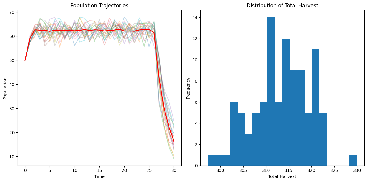
# Plot results
import matplotlib.pyplot as plt
plt.figure(figsize=(12, 6))
plt.subplot(121)
for traj in trajectories[:20]: # Plot first 20 trajectories
plt.plot(range(T+1), traj, alpha=0.3)
plt.plot(range(T+1), avg_trajectory, 'r-', linewidth=2)
plt.title('Population Trajectories')
plt.xlabel('Time')
plt.ylabel('Population')
plt.subplot(122)
plt.hist([sum(h) for h in harvests], bins=20)
plt.title('Distribution of Total Harvest')
plt.xlabel('Total Harvest')
plt.ylabel('Frequency')
plt.tight_layout()
plt.show()
Optimal policy (first few rows):
[[0.  0.  0.  0.  0.  0.  0.  0.  0.  0.  0.  0.  0.  0.  0.  0.  0.  0.
  0.  0.  0.  0.  0.  0.  0.  0.  0.  0.  0.  0.  0.  0.  0.  0.  0.  0.
  0.  0.  0.  0.  0.  0.  0.  0.  0.  0.  0.  0.  0.  0.  0.  0.  0.  0.
  0.  0.1 0.1 0.1 0.1 0.1 0.1 0.1 0.2 0.2 0.2 0.2 0.2 0.2 0.2 0.2 0.2 0.3
  0.3 0.3 0.3 0.3 0.3 0.3 0.3 0.3 0.3 0.3 0.3 0.3 0.4 0.4 0.4 0.4 0.4 0.4
  0.4 0.4 0.4 0.4 0.4 0.4 0.4 0.4 0.4 0.4]
 [0.  0.  0.  0.  0.  0.  0.  0.  0.  0.  0.  0.  0.  0.  0.  0.  0.  0.
  0.  0.  0.  0.  0.  0.  0.  0.  0.  0.  0.  0.  0.  0.  0.  0.  0.  0.
  0.  0.  0.  0.  0.  0.  0.  0.  0.  0.  0.  0.  0.  0.  0.  0.  0.  0.
  0.  0.1 0.1 0.1 0.1 0.1 0.1 0.1 0.2 0.2 0.2 0.2 0.2 0.2 0.2 0.2 0.2 0.3
  0.3 0.3 0.3 0.3 0.3 0.3 0.3 0.3 0.3 0.3 0.3 0.3 0.4 0.4 0.4 0.4 0.4 0.4
  0.4 0.4 0.4 0.4 0.4 0.4 0.4 0.4 0.4 0.4]]

Average population trajectory: [50.         59.126      62.69619476 62.50888039 62.47469976 62.03661246
 62.53917782 62.49630981 62.52289919 62.39429827 62.6029934  62.3916502
 62.81830013 62.4175036  62.67827868 62.5822419  62.18842845 62.41458732
 62.58263582 62.98740346 62.17142674 62.18879702 62.0832301  62.62570881
 62.85043722 62.78845198 61.44489905 42.63269697 30.2230333  22.26564984
 16.40866945]
Average total harvest: 313.43165025164313
Linear Quadratic Regulator via Dynamic Programming#
We now examine a special case where the backward recursion admits a remarkable closed-form solution. When the system dynamics are linear and the cost function is quadratic, the optimization at each stage can be solved analytically. Moreover, the value function itself maintains a quadratic structure throughout the recursion, and the optimal policy reduces to a simple linear feedback law. This elegant result eliminates the need for discretization, interpolation, or any function approximation. The infinite-dimensional problem collapses to tracking a finite set of matrices.
Consider a discrete-time linear system:
where \(\mathbf{x}_t \in \mathbb{R}^n\) is the state and \(\mathbf{u}_t \in \mathbb{R}^m\) is the control input. The matrices \(A_t \in \mathbb{R}^{n \times n}\) and \(B_t \in \mathbb{R}^{n \times m}\) describe the system dynamics at time \(t\).
The cost function to be minimized is quadratic:
where \(Q_T \succeq 0\) (positive semidefinite), \(Q_t \succeq 0\), and \(R_t \succ 0\) (positive definite) are symmetric matrices of appropriate dimensions. The positive definiteness of \(R_t\) ensures the minimization problem is well-posed.
What we now have to observe is that if the terminal cost is quadratic, then the value function at every earlier stage remains quadratic. This is not immediately obvious, but it follows from the structure of Bellman’s equation combined with the linearity of the dynamics.
We claim that the optimal cost-to-go from any stage \(t\) takes the form:
for some positive semidefinite matrix \(P_t\). At the terminal time, this is true by definition: \(P_T = Q_T\).
Let’s verify this structure and derive the recursion for \(P_t\) using backward induction. Suppose we’ve established that \(J_{t+1}^\star(\mathbf{x}_{t+1}) = \frac{1}{2}\mathbf{x}_{t+1}^\top P_{t+1} \mathbf{x}_{t+1}\). Bellman’s equation at stage \(t\) states:
Substituting the dynamics \(\mathbf{x}_{t+1} = A_t\mathbf{x}_t + B_t\mathbf{u}_t\) and the quadratic form for \(J_{t+1}^\star\):
Expanding the last term:
The expression inside the minimization becomes:
Collecting terms involving \(\mathbf{u}_t\):
This is a quadratic function of \(\mathbf{u}_t\). To find the minimizer, we take the gradient with respect to \(\mathbf{u}_t\) and set it to zero:
Since \(R_t + B_t^\top P_{t+1} B_t\) is positive definite (both \(R_t\) and \(P_{t+1}\) are positive semidefinite with \(R_t\) strictly positive), we can solve for the optimal control:
Define the gain matrix:
so that \(\mathbf{u}_t^\star = -K_t\mathbf{x}_t\). This is a linear feedback policy: the optimal control is simply a linear function of the current state.
Substituting \(\mathbf{u}_t^\star\) back into the cost-to-go expression and simplifying (by completing the square), we obtain:
where \(P_t\) satisfies the discrete-time Riccati equation:
Putting everything together, the backward induction procedure under the LQR setting then becomes:
Algorithm 6 (Backward Recursion for LQR)
Input: System matrices \(A_t, B_t\), cost matrices \(Q_t, R_t, Q_T\), time horizon \(T\)
Output: Cost matrices \(P_t\) and gain matrices \(K_t\) for \(t = 0, \ldots, T-1\)
Initialize: \(P_T = Q_T\)
For \(t = T-1, T-2, \ldots, 0\):
Compute the gain matrix:
\[K_t = (R_t + B_t^\top P_{t+1} B_t)^{-1} B_t^\top P_{t+1} A_t\]Compute the cost matrix via the Riccati equation:
\[P_t = Q_t + A_t^\top P_{t+1} A_t - A_t^\top P_{t+1} B_t (R_t + B_t^\top P_{t+1} B_t)^{-1} B_t^\top P_{t+1} A_t\]
End For
Return: \(\{P_0, \ldots, P_T\}\) and \(\{K_0, \ldots, K_{T-1}\}\)
Optimal policy: \(\mathbf{u}_t^\star = -K_t\mathbf{x}_t\)
Optimal cost-to-go: \(J_t^\star(\mathbf{x}_t) = \frac{1}{2}\mathbf{x}_t^\top P_t \mathbf{x}_t\)
Markov Decision Process Formulation#
Rather than expressing the stochasticity in our system through a disturbance term as a parameter to a deterministic difference equation, we often work with an alternative representation (more common in operations research) which uses the Markov Decision Process formulation. The idea is that when we model our system in this way with the disturbance term being drawn indepently of the previous stages, the induced trajectory are those of a Markov chain. Hence, we can re-cast our control problem in that language, leading to the so-called Markov Decision Process framework in which we express the system dynamics in terms of transition probabilities rather than explicit state equations. In this framework, we express the probability that the system is in a given state using the transition probability function:
This function gives the probability of transitioning to state \(\mathbf{x}_{t+1}\) at time \(t+1\), given that the system is in state \(\mathbf{x}_t\) and action \(\mathbf{u}_t\) is taken at time \(t\). Therefore, \(p_t\) specifies a conditional probability distribution over the next states: namely, the sum (for discrete state spaces) or integral over the next state should be 1.
Given the control theory formulation of our problem via a deterministic dynamics function and a noise term, we can derive the corresponding transition probability function through the following relationship:
Here, \(q_t(\mathbf{w})\) represents the probability density or mass function of the disturbance \(\mathbf{W}_t\) (assuming discrete state spaces). When dealing with continuous spaces, the above expression simply contains an integral rather than a summation.
For a system with deterministic dynamics and no disturbance, the transition probabilities become much simpler and be expressed using the indicator function. Given a deterministic system with dynamics:
The transition probability function can be expressed as:
With this transition probability function, we can recast our Bellman optimality equation:
Here, \({c}(\mathbf{x}_t, \mathbf{u}_t)\) represents the expected immediate reward (or negative cost) when in state \(\mathbf{x}_t\) and taking action \(\mathbf{u}_t\) at time \(t\). The summation term computes the expected optimal value for the future states, weighted by their transition probabilities.
This formulation offers several advantages:
It makes the Markovian nature of the problem explicit: the future state depends only on the current state and action, not on the history of states and actions.
For discrete-state problems, the entire system dynamics can be specified by a set of transition matrices, one for each possible action.
It allows us to bridge the gap with the wealth of methods in the field of probabilistic graphical models and statistical machine learning techniques for modelling and analysis.
Notation in Operations Reseach#
The presentation above was intended to bridge the gap between the control-theoretic perspective and the world of closed-loop control through the idea of determining the value function of a parametric optimal control problem. We then saw how the backward induction procedure was applicable to both the deterministic and stochastic cases by taking the expectation over the disturbance variable. We then said that we can alternatively work with a representation of our system where instead of writing our model as a deterministic dynamics function taking a disturbance as an input, we would rather work directly via its transition probability function, which gives rise to the Markov chain interpretation of our system in simulation.
Now we should highlight that the notation used in control theory tends to differ from that found in operations research communities, in which the field of dynamic programming flourished. We summarize those (purely notational) differences in this section.
In operations research, the system state at each decision epoch is typically denoted by \(s \in \mathcal{S}\), where \(S\) is the set of possible system states. When the system is in state \(s\), the decision maker may choose an action \(a\) from the set of allowable actions \(\mathcal{A}_s\). The union of all action sets is denoted as \(\mathcal{A} = \bigcup_{s \in \mathcal{S}} \mathcal{A}_s\).
The dynamics of the system are described by a transition probability function \(p_t(j | s, a)\), which represents the probability of transitioning to state \(j \in \mathcal{S}\) at time \(t+1\), given that the system is in state \(s\) at time \(t\) and action \(a \in \mathcal{A}_s\) is chosen. This transition probability function satisfies:
It’s worth noting that in operations research, we typically work with reward maximization rather than cost minimization, which is more common in control theory. However, we can easily switch between these perspectives by simply negating the quantity. That is, maximizing a reward function is equivalent to minimizing its negative, which we would then call a cost function.
The reward function is denoted by \(r_t(s, a)\), representing the reward received at time \(t\) when the system is in state \(s\) and action \(a\) is taken. In some cases, the reward may also depend on the next state, in which case it is denoted as \(r_t(s, a, j)\). The expected reward can then be computed as:
Combined together, these elemetns specify a Markov decision process, which is fully described by the tuple:
where \(\mathrm{T}\) represents the set of decision epochs (the horizon).
What is an Optimal Policy?#
Let’s go back to the starting point and define what it means for a policy to be optimal in a Markov Decision Problem. For this, we will be considering different possible search spaces (policy classes) and compare policies based on the ordering of their value from any possible start state. The value of a policy \(\boldsymbol{\pi}\) (optimal or not) is defined as the expected total reward obtained by following that policy from a given starting state. Formally, for a finite-horizon MDP with \(N\) decision epochs, we define the value function \(v^{\boldsymbol{\pi}}(s, t)\) as:
where \(S_t\) is the state at time \(t\), \(A_t\) is the action taken at time \(t\), and \(r_t\) is the reward function. For simplicity, we write \(v^{\boldsymbol{\pi}}(s)\) to denote \(v^{\boldsymbol{\pi}}(s, 1)\), the value of following policy \(\boldsymbol{\pi}\) from state \(s\) at the first stage over the entire horizon \(N\).
In finite-horizon MDPs, our goal is to identify an optimal policy, denoted by \(\boldsymbol{\pi}^*\), that maximizes total expected reward over the horizon \(N\). Specifically:
We call \(\boldsymbol{\pi}^*\) an optimal policy because it yields the highest possible value across all states and all policies within the policy class \(\Pi^{\text{HR}}\). We denote by \(v^*\) the maximum value achievable by any policy:
In reinforcement learning literature, \(v^*\) is typically referred to as the “optimal value function,” while in some operations research references, it might be called the “value of an MDP.” An optimal policy \(\boldsymbol{\pi}^*\) is one for which its value function equals the optimal value function:
This notion of optimality applies to every state. Policies optimal in this sense are sometimes called “uniformly optimal policies.” A weaker notion of optimality, often encountered in reinforcement learning practice, is optimality with respect to an initial distribution of states. In this case, we seek a policy \(\boldsymbol{\pi} \in \Pi^{\text{HR}}\) that maximizes:
where \(P_1(S_1 = s)\) is the probability of starting in state \(s\).
The maximum value can be achieved by searching over the space of deterministic Markovian Policies. Consequently:
This equality significantly simplifies the computational complexity of our algorithms, as the search problem can now be decomposed into \(N\) sub-problems in which we only have to search over the set of possible actions. This is the backward induction algorithm, which we present a second time, but departing this time from the control-theoretic notation and using the MDP formalism:
Algorithm 7 (Backward Induction)
Input: State space \(S\), Action space \(A\), Transition probabilities \(p_t\), Reward function \(r_t\), Time horizon \(N\)
Output: Optimal value functions \(v^*\)
Initialize:
Set \(t = N\)
For all \(s_N \in S\):
\[v^*(s_N, N) = r_N(s_N)\]
For \(t = N-1\) to \(1\):
For each \(s_t \in S\): a. Compute the optimal value function:
\[v^*(s_t, t) = \max_{a \in A_{s_t}} \left\{r_t(s_t, a) + \sum_{j \in S} p_t(j | s_t, a) v^*(j, t+1)\right\}\]b. Determine the set of optimal actions:
\[A_{s_t,t}^* = \arg\max_{a \in A_{s_t}} \left\{r_t(s_t, a) + \sum_{j \in S} p_t(j | s_t, a) v^*(j, t+1)\right\}\]
Return the optimal value functions \(u_t^*\) and optimal action sets \(A_{s_t,t}^*\) for all \(t\) and \(s_t\)
Note that the same procedure can also be used for finding the value of a policy with minor changes;
Algorithm 8 (Policy Evaluation)
Input:
State space \(S\)
Action space \(A\)
Transition probabilities \(p_t\)
Reward function \(r_t\)
Time horizon \(N\)
A markovian deterministic policy \(\boldsymbol{\pi} = (\pi_1, \ldots, \pi_{N-1})\)
Output: Value function \(v^{\boldsymbol{\pi}}\) for policy \(\boldsymbol{\pi}\)
Initialize:
Set \(t = N\)
For all \(s_N \in S\):
\[v^{\boldsymbol{\pi}}(s_N, N) = r_N(s_N)\]
For \(t = N-1\) to \(1\):
For each \(s_t \in S\): a. Compute the value function for the given policy:
\[v^{\boldsymbol{\pi}}(s_t, t) = r_t(s_t, \pi_t(s_t)) + \sum_{j \in S} p_t(j | s_t, \pi_t(s_t)) v^{\boldsymbol{\pi}}(j, t+1)\]
Return the value function \(v^{\boldsymbol{\pi}}(s_t, t)\) for all \(t\) and \(s_t\)
This code could also finally be adapted to support randomized policies using:
Example: Sample Size Determination in Pharmaceutical Development#
Pharmaceutical development is the process of bringing a new drug from initial discovery to market availability. This process is lengthy, expensive, and risky, typically involving several stages:
Drug Discovery: Identifying a compound that could potentially treat a disease.
Preclinical Testing: Laboratory and animal testing to assess safety and efficacy. . Clinical Trials: Testing the drug in humans, divided into phases:
Phase I: Testing for safety in a small group of healthy volunteers.
Phase II: Testing for efficacy and side effects in a larger group with the target condition.
Phase III: Large-scale testing to confirm efficacy and monitor side effects.
Regulatory Review: Submitting a New Drug Application (NDA) for approval.
Post-Market Safety Monitoring: Continuing to monitor the drug’s effects after market release.
This process can take 10-15 years and cost over $1 billion [1]. The high costs and risks involved call for a principled approach to decision making. We’ll focus on the clinical trial phases and NDA approval, per the MDP model presented by [6]:
States (\(S\)): Our state space is \(S = \{s_1, s_2, s_3, s_4\}\), where:
\(s_1\): Phase I clinical trial
\(s_2\): Phase II clinical trial
\(s_3\): Phase III clinical trial
\(s_4\): NDA approval
Actions (\(A\)): At each state, the action is choosing the sample size \(n_i\) for the corresponding clinical trial. The action space is \(A = \{10, 11, ..., 1000\}\), representing possible sample sizes.
Transition Probabilities (\(P\)): The probability of moving from one state to the next depends on the chosen sample size and the inherent properties of the drug. We define:
\(P(s_2|s_1, n_1) = p_{12}(n_1) = \sum_{i=0}^{\lfloor\eta_1 n_1\rfloor} \binom{n_1}{i} p_0^i (1-p_0)^{n_1-i}\) where \(p_0\) is the true toxicity rate and \(\eta_1\) is the toxicity threshold for Phase I.
Of particular interest is the transition from Phase II to Phase III which we model as:
\(P(s_3|s_2, n_2) = p_{23}(n_2) = \Phi\left(\frac{\sqrt{n_2}}{2}\delta - z_{1-\eta_2}\right)\)
where \(\Phi\) is the cumulative distribution function (CDF) of the standard normal distribution:
\(\Phi(x) = \frac{1}{\sqrt{2\pi}} \int_{-\infty}^x e^{-t^2/2} dt\)
This is giving us the probability that we would observe a treatment effect this large or larger if the null hypothesis (no treatment effect) were true. A higher probability indicates stronger evidence of a treatment effect, making it more likely that the drug will progress to Phase III.
In this expression, \(\delta\) is called the “normalized treatment effect”. In clinical trials, we’re often interested in the difference between the treatment and control groups. The “normalized” part means we’ve adjusted this difference for the variability in the data. Specifically \(\delta = \frac{\mu_t - \mu_c}{\sigma}\) where \(\mu_t\) is the mean outcome in the treatment group, \(\mu_c\) is the mean outcome in the control group, and \(\sigma\) is the standard deviation of the outcome. A larger \(\delta\) indicates a stronger treatment effect.
Furthermore, the term \(z_{1-\eta_2}\) is the \((1-\eta_2)\)-quantile of the standard normal distribution. In other words, it’s the value where the probability of a standard normal random variable being greater than this value is \(\eta_2\). For example, if \(\eta_2 = 0.05\), then \(z_{1-\eta_2} \approx 1.645\). A smaller \(\eta_2\) makes the trial more conservative, requiring stronger evidence to proceed to Phase III.
Finally, \(n_2\) is the sample size for Phase II. The \(\sqrt{n_2}\) term reflects that the precision of our estimate of the treatment effect improves with the square root of the sample size.
\(P(s_4|s_3, n_3) = p_{34}(n_3) = \Phi\left(\frac{\sqrt{n_3}}{2}\delta - z_{1-\eta_3}\right)\) where \(\eta_3\) is the significance level for Phase III.
Rewards (\(R\)): The reward function captures the costs of running trials and the potential profit from a successful drug:
\(r(s_i, n_i) = -c_i(n_i)\) for \(i = 1, 2, 3\), where \(c_i(n_i)\) is the cost of running a trial with sample size \(n_i\).
\(r(s_4) = g_4\), where \(g_4\) is the expected profit from a successful drug.
Discount Factor (\(\gamma\)): We use a discount factor \(0 < \gamma \leq 1\) to account for the time value of money and risk preferences.
Show code cell source
import numpy as np
from scipy.stats import binom
from scipy.stats import norm

def binomial_pmf(k, n, p):
    return binom.pmf(k, n, p)

def transition_prob_phase1(n1, eta1, p0):
    return np.sum([binomial_pmf(i, n1, p0) for i in range(int(eta1 * n1) + 1)])

def transition_prob_phase2(n2, eta2, delta):
    return norm.cdf((np.sqrt(n2) / 2) * delta - norm.ppf(1 - eta2))

def transition_prob_phase3(n3, eta3, delta):
    return norm.cdf((np.sqrt(n3) / 2) * delta - norm.ppf(1 - eta3))

def immediate_reward(n):
    return -n  # Negative to represent cost

def backward_induction(S, A, gamma, g4, p0, delta, eta1, eta2, eta3):
    V = np.zeros(len(S))
    V[3] = g4  # Value for NDA approval state
    optimal_n = [None] * 3  # Store optimal n for each phase

    # Backward induction
    for i in range(2, -1, -1):  # Iterate backwards from Phase III to Phase I
        max_value = -np.inf
        for n in A:
            if i == 0:  # Phase I
                p = transition_prob_phase1(n, eta1, p0)
            elif i == 1:  # Phase II
                p = transition_prob_phase2(n, eta2, delta)
            else:  # Phase III
                p = transition_prob_phase3(n, eta3, delta)
            value = immediate_reward(n) + gamma * p * V[i+1]
            if value > max_value:
                max_value = value
                optimal_n[i] = n
        V[i] = max_value

    return V, optimal_n

# Set up the problem parameters
S = ['Phase I', 'Phase II', 'Phase III', 'NDA approval']
A = range(10, 1001)
gamma = 0.95
g4 = 10000
p0 = 0.1  # Example toxicity rate for Phase I
delta = 0.5  # Example normalized treatment difference
eta1, eta2, eta3 = 0.2, 0.1, 0.025

# Run the backward induction algorithm
V, optimal_n = backward_induction(S, A, gamma, g4, p0, delta, eta1, eta2, eta3)

# Print results
for i, state in enumerate(S):
    print(f"Value for {state}: {V[i]:.2f}")
print(f"Optimal sample sizes: Phase I: {optimal_n[0]}, Phase II: {optimal_n[1]}, Phase III: {optimal_n[2]}")

# Sanity checks
print("\nSanity checks:")
print(f"1. NDA approval value: {V[3]}")
print(f"2. All values non-positive and <= NDA value: {all(v <= V[3] for v in V)}")
print(f"3. Optimal sample sizes in range: {all(10 <= n <= 1000 for n in optimal_n if n is not None)}")
Value for Phase I: 7869.92
Value for Phase II: 8385.83
Value for Phase III: 9123.40
Value for NDA approval: 10000.00
Optimal sample sizes: Phase I: 75, Phase II: 239, Phase III: 326

Sanity checks:
1. NDA approval value: 10000.0
2. All values non-positive and <= NDA value: True
3. Optimal sample sizes in range: True
Infinite-Horizon MDPs#
It often makes sense to model control problems over infinite horizons. We extend the previous setting and define the expected total reward of policy \(\boldsymbol{\pi} \in \Pi^{\mathrm{HR}}\), \(v^{\boldsymbol{\pi}}\) as:
One drawback of this model is that we could easily encounter values that are \(+\infty\) or \(-\infty\), even in a setting as simple as a single-state MDP which loops back into itself and where the accrued reward is nonzero.
Therefore, it is often more convenient to work with an alternative formulation which guarantees the existence of a limit: the expected total discounted reward of policy \(\boldsymbol{\pi} \in \Pi^{\mathrm{HR}}\) is defined to be:
for \(0 \leq \gamma < 1\) and when \(\max_{s \in \mathcal{S}} \max_{a \in \mathcal{A}_s}|r(s, a)| = R_{\max} < \infty\), in which case, \(|v_\gamma^{\boldsymbol{\pi}}(s)| \leq (1-\gamma)^{-1} R_{\max}\).
Finally, another possibility for the infinite-horizon setting is the so-called average reward or gain of policy \(\boldsymbol{\pi} \in \Pi^{\mathrm{HR}}\) defined as:
We won’t be working with this formulation in this course due to its inherent practical and theoretical complexities.
Extending the previous notion of optimality from finite-horizon models, a policy \(\boldsymbol{\pi}^*\) is said to be discount optimal for a given \(\gamma\) if:
Furthermore, the value of a discounted MDP \(v_\gamma^*(s)\), is defined by:
More often, we refer to \(v_\gamma\) by simply calling it the optimal value function.
As for the finite-horizon setting, the infinite horizon discounted model does not require history-dependent policies, since for any \(\boldsymbol{\pi} \in \Pi^{HR}\) there exists a \(\boldsymbol{\pi}^{\prime} \in \Pi^{MR}\) with identical total discounted reward: $\( v_\gamma^*(s) \equiv \max_{\boldsymbol{\pi} \in \Pi^{HR}} v_\gamma^{\boldsymbol{\pi}}(s)=\max_{\boldsymbol{\pi} \in \Pi^{MR}} v_\gamma^{\boldsymbol{\pi}}(s) . \)$
Random Horizon Interpretation of Discounting#
The use of discounting can be motivated both from a modeling perspective and as a means to ensure that the total reward remains bounded. From the modeling perspective, we can view discounting as a way to weight more or less importance on the immediate rewards vs. the long-term consequences. There is also another interpretation which stems from that of a finite horizon model but with an uncertain end time. More precisely:
Let \(v_\nu^{\boldsymbol{\pi}}(s)\) denote the expected total reward obtained by using policy \(\boldsymbol{\pi}\) when the horizon length \(\nu\) is random. We define it by:
Theorem 5 (Random horizon interpretation of discounting)
Suppose that the horizon \(\nu\) follows a geometric distribution with parameter \(\gamma\), \(0 \leq \gamma < 1\), independent of the policy such that \(P(\nu=n) = (1-\gamma) \gamma^{n-1}, \, n=1,2, \ldots\), then \(v_\nu^{\boldsymbol{\pi}}(s) = v_\gamma^{\boldsymbol{\pi}}(s)\) for all \(s \in \mathcal{S}\) .
Proof. See proposition 5.3.1 in [34].
By definition of the finite-horizon value function and the law of total expectation:
Combining the expectation with the sum over \(n\):
Reordering the summations: Under the bounded reward assumption \(|r(s,a)| \leq R_{\max}\) and \(\gamma < 1\), we have
which justifies exchanging the order of summation by Fubini’s theorem.
To reverse the order, note that the pair \((n,t)\) with \(1 \leq t \leq n\) can be reindexed by fixing \(t\) first and letting \(n\) range from \(t\) to \(\infty\):
Therefore:
Evaluating the inner sum: Using the substitution \(m = n - t + 1\) (so \(n = m + t - 1\)):
Substituting back:
Vector Representation in Markov Decision Processes#
Let V be the set of bounded real-valued functions on a discrete state space S. This means any function \( f \in V \) satisfies the condition:
where notation \( \|f\| \) represents the sup-norm (or \( \ell_\infty \)-norm) of the function \( f \).
When working with discrete state spaces, we can interpret elements of V as vectors and linear operators on V as matrices, allowing us to leverage tools from linear algebra. The sup-norm (\(\ell_\infty\) norm) of matrix \(\mathbf{H}\) is defined as:
where \(\mathbf{H}_{s,j}\) represents the \((s, j)\)-th component of the matrix \(\mathbf{H}\).
For a Markovian decision rule \(\pi \in \Pi^{MD}\), we define:
For a randomized decision rule \(\pi \in \Pi^{MR}\), these definitions extend to:
In both cases, \(\mathbf{r}_\pi\) denotes a reward vector in \(\mathbb{R}^{|S|}\), with each component \(\mathbf{r}_\pi(s)\) representing the reward associated with state \(s\). Similarly, \(\mathbf{P}_\pi\) is a transition probability matrix in \(\mathbb{R}^{|S| \times |S|}\), capturing the transition probabilities under decision rule \(\pi\).
For a nonstationary Markovian policy \(\boldsymbol{\pi} = (\pi_1, \pi_2, \ldots) \in \Pi^{MR}\), the expected total discounted reward is given by:
Using vector notation, this can be expressed as:
This formulation leads to a recursive relationship:
where \(\boldsymbol{\pi}^{\prime} = (\pi_2, \pi_3, \ldots)\).
For a stationary policy \(\boldsymbol{\pi} = \mathrm{const}(\pi)\) with constant decision rule \(\pi\), the total expected reward simplifies to:
This last expression is called a Neumann series expansion, and it’s guaranteed to exists under the assumptions of bounded reward and discount factor strictly less than one.
Theorem 6 (Neumann Series and Invertibility)
The spectral radius of a matrix \(\mathbf{H}\) is defined as:
where \(\lambda_i(\mathbf{H})\) are the eigenvalues of \(\mathbf{H}\).
Neumann Series Existence: For any matrix \(\mathbf{H}\), the Neumann series
converges if and only if \(\rho(\mathbf{H}) < 1\). When this condition holds, the matrix \((\mathbf{I} - \mathbf{H})\) is invertible and
Note that for any induced matrix norm \(\|\cdot\|\) (i.e., a norm satisfying \(\|\mathbf{H}\mathbf{v}\| \leq \|\mathbf{H}\| \cdot \|\mathbf{v}\|\) for all vectors \(\mathbf{v}\)) and any matrix \(\mathbf{H}\), the spectral radius is bounded by:
This inequality provides a practical way to verify the convergence condition \(\rho(\mathbf{H}) < 1\) by checking the simpler condition \(\|\mathbf{H}\| < 1\) rather than trying to compute the eigenvalues directly.
We can now verify that \((\mathbf{I} - \gamma \mathbf{P}_d)\) is invertible and the Neumann series converges.
Norm of the transition matrix: Since \(\mathbf{P}_d\) is a stochastic matrix (each row sums to 1 and all entries are non-negative), its \(\ell_\infty\)-norm is:
\[ \|\mathbf{P}_d\| = \max_{s \in S} \sum_{j \in S} [\mathbf{P}_d]_{s,j} = \max_{s \in S} 1 = 1. \]Norm of the scaled matrix: Using the homogeneity property of norms, we have:
\[ \|\gamma \mathbf{P}_d\| = |\gamma| \cdot \|\mathbf{P}_d\| = |\gamma| \cdot 1 = |\gamma|. \]Bounding the spectral radius: Since the spectral radius is bounded by the matrix norm:
\[ \rho(\gamma \mathbf{P}_d) \leq \|\gamma \mathbf{P}_d\| = |\gamma|. \]Verifying convergence: Since \(0 \leq \gamma < 1\) by assumption, we have:
\[ \rho(\gamma \mathbf{P}_d) \leq |\gamma| < 1. \]This strict inequality guarantees that \((\mathbf{I} - \gamma \mathbf{P}_d)\) is invertible and the Neumann series converges.
Therefore, the Neumann series expansion converges and yields:
Consequently, for a stationary policy, \(\mathbf{v}_\gamma^{d^\infty}\) can be determined as the solution to the linear equation:
which can be rearranged to:
We can also characterize \(\mathbf{v}_\gamma^{d^\infty}\) as the solution to an operator equation. More specifically, define the transformation \(\mathrm{L}_d\) by
for any \(\mathbf{v} \in V\). Intuitively, \(\mathrm{L}_d\) takes a value function \(\mathbf{v}\) as input and returns a new value function that combines immediate rewards (\(\mathbf{r}_d\)) with discounted future values (\(\gamma \mathbf{P}_d\mathbf{v}\)).
Note
While we often refer to \(\mathrm{L}_d\) as a “linear operator” in the RL literature, it is technically an affine operator (or affine transformation), not a linear operator in the strict sense. To see why, recall that a linear operator \(\mathcal{T}\) must satisfy:
Additivity: \(\mathcal{T}(\mathbf{v}_1 + \mathbf{v}_2) = \mathcal{T}(\mathbf{v}_1) + \mathcal{T}(\mathbf{v}_2)\)
Homogeneity: \(\mathcal{T}(\alpha \mathbf{v}) = \alpha \mathcal{T}(\mathbf{v})\) for all scalars \(\alpha\)
However, \(\mathrm{L}_d\) fails the additivity test:
while
The presence of the constant term \(\mathbf{r}_d\) makes \(\mathrm{L}_d\) affine rather than linear. An affine operator has the form \(\mathcal{A}(\mathbf{v}) = \mathbf{b} + \mathcal{T}(\mathbf{v})\), where \(\mathbf{b}\) is a constant vector and \(\mathcal{T}\) is a linear operator. In our case, \(\mathbf{b} = \mathbf{r}_d\) and \(\mathcal{T}(\mathbf{v}) = \gamma \mathbf{P}_d\mathbf{v}\).
Despite this technical distinction, the term “linear operator” is commonly used in the reinforcement learning literature when referring to \(\mathrm{L}_d\), following a slight abuse of terminology.
Therefore, we view \(\mathrm{L}_d\) as an operator mapping elements of \(V\) to \(V\): i.e., \(\mathrm{L}_d: V \rightarrow V\). The fact that the value function of a policy is the solution to a fixed-point equation can then be expressed with the statement:
This is a fixed-point equation: the value function \(\mathbf{v}_\gamma^{d^\infty}\) is a fixed point of the operator \(\mathrm{L}_d\).
Solving Operator Equations#
The operator equation we encountered in MDPs, \(\mathbf{v}_\gamma^{d^\infty} = \mathrm{L}_d \mathbf{v}_\gamma^{d^\infty}\), is a specific instance of a more general class of problems known as operator equations. These equations appear in various fields of mathematics and applied sciences, ranging from differential equations to functional analysis.
Operator equations can take several forms, each with its own characteristics and solution methods:
Fixed Point Form: \(x = \mathrm{T}(x)\), where \(\mathrm{T}: X \rightarrow X\). Common in fixed-point problems, such as our MDP equation, we seek a fixed point \(x^*\) such that \(x^* = \mathrm{T}(x^*)\).
General Operator Equation: \(\mathrm{T}(x) = y\), where \(\mathrm{T}: X \rightarrow Y\). Here, \(X\) and \(Y\) can be different spaces. We seek an \(x \in X\) that satisfies the equation for a given \(y \in Y\).
Nonlinear Equation: \(\mathrm{T}(x) = 0\), where \(\mathrm{T}: X \rightarrow Y\). A special case of the general operator equation where we seek roots or zeros of the operator.
Variational Inequality: Find \(x^* \in K\) such that \(\langle \mathrm{T}(x^*), x - x^* \rangle \geq 0\) for all \(x \in K\). Here, \(K\) is a closed convex subset of \(X\), and \(\mathrm{T}: K \rightarrow X^*\) (the dual space of \(X\)). These problems often arise in optimization, game theory, and partial differential equations.
Successive Approximation Method#
For equations in fixed point form, a common numerical solution method is successive approximation, also known as fixed-point iteration:
Algorithm 9 (Successive Approximation)
Input: An operator \(\mathrm{T}: X \rightarrow X\), an initial guess \(x_0 \in X\), and a tolerance \(\epsilon > 0\)
Output: An approximate fixed point \(x^*\) such that \(\|x^* - \mathrm{T}(x^*)\| < \epsilon\)
Initialize \(n = 0\)
repeat
3. Compute \(x_{n+1} = \mathrm{T}(x_n)\)
4. If \(\|x_{n+1} - x_n\| < \epsilon\), return \(x_{n+1}\)
5. Set \(n = n + 1\)until convergence or maximum iterations reached
The convergence of successive approximation depends on the properties of the operator \(\mathrm{T}\). In the simplest and most common setting, we assume \(\mathrm{T}\) is a contraction mapping. The Banach Fixed-Point Theorem then guarantees that \(\mathrm{T}\) has a unique fixed point, and the successive approximation method will converge to this fixed point from any starting point. Specifically, \(\mathrm{T}\) is a contraction if there exists a constant \(q \in [0,1)\) such that for all \(x,y \in X\):
where \(d\) is the metric on \(X\). In this case, the rate of convergence is linear, with error bound:
However, the contraction mapping condition is not the only one that can lead to convergence. For instance, if \(\mathrm{T}\) is nonexpansive (i.e., Lipschitz continuous with Lipschitz constant 1) and \(X\) is a Banach space with certain geometrical properties (e.g., uniformly convex), then under additional conditions (e.g., \(\mathrm{T}\) has at least one fixed point), the successive approximation method can still converge, albeit potentially more slowly than in the contraction case.
In practice, when dealing with specific problems like MDPs or differential equations, the properties of the operator often naturally align with one of these convergence conditions. For example, in discounted MDPs, the Bellman operator is a contraction in the supremum norm, which guarantees the convergence of value iteration.
Newton-Kantorovich Method#
The Newton-Kantorovich method is a generalization of Newton’s method from finite dimensional vector spaces to infinite dimensional function spaces: rather than iterating in the space of vectors, we are iterating in the space of functions.
Newton’s method is often written as the familiar update:
which makes it look as though the essence of the method is “take a derivative and invert it.” But the real workhorse behind Newton’s method (both in finite and infinite dimensions) is linearization.
At each step, the idea is to replace the nonlinear operator \(F:X \to Y\) by a local surrogate model of the form
where \(L\) is a linear map capturing how small perturbations in the input propagate to changes in the output. This is a Taylor-like expansion in Banach spaces: the role of the derivative is precisely to provide the correct notion of such a linear operator.
To find a root of \(F\), we impose the condition that the surrogate vanishes at the next iterate:
Solving this linear equation gives the increment \(h\). In finite dimensions, \(L\) is the Jacobian matrix; in Banach spaces, it must be the Fréchet derivative.
But what exactly is a Fréchet derivative in infinite dimensions? To understand this, we need to generalize the concept of derivative from finite-dimensional calculus. In infinite-dimensional spaces, there are several notions of differentiability, each with different strengths and requirements:
1. Gâteaux (Directional) Derivative
We say that the Gâteaux derivative of \(F\) at \(x\) in a specific direction \(h\) is:
This quantity measures how the function \(F\) changes along the ray \(x + th\). While this limit may exist for each direction \(h\) separately, it doesn’t guarantee that the derivative is linear in \(h\). This is a key limitation: the Gâteaux derivative can exist in all directions but still fail to provide a good linear approximation.
2. Hadamard Directional Derivative
Rather than considering a single direction of perturbation, we now consider a bundle of perturbations around \(h\). We ask how the function changes as we approach the target direction from nearby directions. We say that \(F\) has a Hadamard directional derivative if:
This is a stronger condition than Gâteaux differentiability because it requires the limit to be uniform over nearby directions. However, it still doesn’t guarantee linearity in \(h\).
3. Fréchet Derivative
The strongest and most natural notion: \(F\) is Fréchet differentiable at \(x\) if there exists a bounded linear operator \(L\) such that:
This definition directly addresses the inadequacy of the previous notions. Unlike Gâteaux and Hadamard derivatives, the Fréchet derivative explicitly requires the existence of a linear operator \(L\) that provides a good approximation. Key properties:
\(L\) must be linear in \(h\) (unlike the directional derivatives above)
The approximation error is \(o(\|h\|)\), uniform in all directions
This is the “true” derivative: it generalizes the Jacobian matrix to infinite dimensions
Notation: \(L = F'(x)\) or \(DF(x)\)
Relationship:
In the context of the Newton-Kantorovich method, we work with an operator \(F: X \to Y\) where both \(X\) and \(Y\) are Banach spaces. The Fréchet derivative \(F'(x)\) is the best linear approximation of \(F\) near \(x\), and it’s exactly this linear operator \(L\) that we use in our linearization \(F(x+h) \approx F(x) + F'(x)h\).
Now apart from those mathematical technicalities, Newton-Kantorovich has in essence the same structure as that of the original Newton’s method. That is, it applies the following sequence of steps:
Linearize the Operator: Given an approximation \( x_n \), we consider the Fréchet derivative of \( F \), denoted by \( F'(x_n) \). This derivative is a linear operator that provides a local approximation of \( F \) near \( x_n \).
Set Up the Newton Step: The method then solves the linearized equation for a correction \( h_n \):
\[ F'(x_n) h_n = -F(x_n). \]This equation represents a linear system where \( h_n \) is chosen so that the linearized operator \( F(x_n) + F'(x_n)h_n \) equals zero.
Update the Solution: The new approximation \( x_{n+1} \) is then given by:
\[ x_{n+1} = x_n + h_n. \]This correction step refines \( x_n \), bringing it closer to the true solution.
Repeat Until Convergence: We repeat the linearization and update steps until the solution \( x_n \) converges to the desired tolerance, which can be verified by checking that \( \|F(x_n)\| \) is sufficiently small, or by monitoring the norm \( \|x_{n+1} - x_n\| \).
The convergence of Newton-Kantorovich does not hinge on \( F \) being a contraction over the entire domain (as it could be the case for successive approximation). The convergence properties of the Newton-Kantorovich method are as follows:
Local Convergence: Under mild conditions (e.g., \(F\) is Fréchet differentiable and \(F'(x)\) is invertible near the solution), the method converges locally. This means that if the initial guess is sufficiently close to the true solution, the method will converge.
Global Convergence: Global convergence is not guaranteed in general. However, under stronger conditions (e.g., \(F\) is analytic and satisfies certain bounds), the method can converge globally.
Rate of Convergence: When the method converges, it typically exhibits quadratic convergence. This means that the error at each step is proportional to the square of the error at the previous step:
\[ \|x_{n+1} - x^*\| \leq C\|x_n - x^*\|^2 \]where \(x^*\) is the true solution and \(C\) is some constant. This quadratic convergence is significantly faster than the linear convergence typically seen in methods like successive approximation.
Optimality Equations for Infinite-Horizon MDPs#
Recall that in the finite-horizon setting, the optimality equations are:
where \(v_n(s)\) is the value function at time step \(n\) for state \(s\), \(A_s\) is the set of actions available in state \(s\), \(r(s, a)\) is the reward function, \(\gamma\) is the discount factor, and \(p(j | s, a)\) is the transition probability from state \(s\) to state \(j\) given action \(a\).
Intuitively, we would expect that by taking the limit of \(n\) to infinity, we might get the nonlinear equations:
which are called the optimality equations or Bellman equations for infinite-horizon MDPs.
We can adopt an operator-theoretic perspective by defining operators on the space \(V\) of bounded real-valued functions on the state space \(S\). For a deterministic Markov rule \(\pi \in \Pi^{MD}\), define the policy-evaluation operator:
The Bellman optimality operator is then:
where \(\Pi^{MD}\) is the set of Markov deterministic decision rules, \(\mathbf{r}_\pi\) is the reward vector under decision rule \(\pi\), and \(\mathbf{P}_\pi\) is the transition probability matrix under decision rule \(\pi\).
Note that while we write \(\max_{\pi \in \Pi^{MD}}\), we do not implement the above operator by enumerating all decision rules. Rather, the fact that we compare policies based on their value functions in a componentwise fashion means that maximizing over the space of Markovian deterministic rules reduces to the following update in component form:
For convenience, we define the greedy selector \(\mathrm{Greedy}(v) \in \Pi^{MD}\) that extracts an optimal decision rule from a value function:
In Puterman’s terminology, such a greedy selector is called \(v\)-improving (or conserving when it achieves the maximum). This operator will be useful for expressing algorithms succinctly:
Value iteration: \(v_{k+1} = \mathrm{L}v_k\), then extract \(\pi = \mathrm{Greedy}(v^*)\)
Policy iteration: \(\pi_{k+1} = \mathrm{Greedy}(v^{\pi_k})\) with \(v^{\pi_k}\) solving \(v = \mathrm{L}_{\pi_k}v\)
The equivalence between these two forms can be shown mathematically, as demonstrated in the following proposition and proof.
Proposition 3
The operator \(\mathrm{L}\) defined as a maximization over Markov deterministic decision rules:
is equivalent to the componentwise maximization over actions:
Proof. Fix \(s\). Let
For any rule \(\pi \in \Pi^{MD}\), we have \((\mathrm{L}_\pi v)(s)=Q_v(s,\pi(s))\le \max_{a\in\mathcal{A}_s}Q_v(s,a)\).
Taking the maximum over \(\pi\) gives
Conversely, choose a greedy selector \(\pi^v\in\Pi^{MD}\) such that for each \(s\),
(possible since \(\mathcal{A}_s\) is finite; otherwise use a measurable \(\varepsilon\)-greedy selector). Then
so \(\max_{\pi}(\mathrm{L}_\pi v)(s)\ge \max_{a}Q_v(s,a)\). Combining both inequalities yields equality.
Algorithms for Solving the Optimality Equations#
The optimality equations are operator equations. Therefore, we can apply general numerical methods to solve them. Applying the successive approximation method to the Bellman optimality equation yields a method known as “value iteration” in dynamic programming. A direct application of the blueprint for successive approximation yields the following algorithm:
Algorithm 10 (Value Iteration)
Input Given an MDP \((S, A, P, R, \gamma)\) and tolerance \(\varepsilon > 0\)
Output Compute an \(\varepsilon\)-optimal value function \(v\) and policy \(\pi\)
Initialize \(v_0(s) = 0\) for all \(s \in S\)
\(n \leftarrow 0\)
repeat
For each \(s \in S\):
\(v_{n+1}(s) \leftarrow (\mathrm{L}v_n)(s) = \max_{a \in A} \left\{r(s,a) + \gamma \sum_{j \in \mathcal{S}} p(j|s,a)v_n(j)\right\}\)
\(\delta \leftarrow \|v_{n+1} - v_n\|_\infty\)
\(n \leftarrow n + 1\)
until \(\delta < \frac{\varepsilon(1-\gamma)}{2\gamma}\)
Extract greedy policy: \(\pi \leftarrow \mathrm{Greedy}(v_n)\) where
\[\mathrm{Greedy}(v)(s) \in \arg\max_{a \in \mathcal{A}_s} \left\{r(s,a) + \gamma \sum_{j \in \mathcal{S}} p(j|s,a)v(j)\right\}\]return \(v_n, \pi\)
The termination criterion in this algorithm is based on a specific bound that provides guarantees on the quality of the solution. This is in contrast to supervised learning, where we often use arbitrary termination criteria based on computational budget or early stopping when the learning curve flattens. This is because establishing implementable generalization bounds in supervised learning is challenging.
However, in the dynamic programming context, we can derive various bounds that can be implemented in practice. These bounds help us terminate our procedure with a guarantee on the precision of our value function and, correspondingly, on the optimality of the resulting policy.
Proposition 4 (Convergence of Value Iteration)
(Adapted from Puterman [34] theorem 6.3.1)
Let \(v_0\) be any initial value function, \(\varepsilon > 0\) a desired accuracy, and let \(\{v_n\}\) be the sequence of value functions generated by value iteration, i.e., \(v_{n+1} = \mathrm{L}v_n\) for \(n \geq 0\), where \(\mathrm{L}\) is the Bellman optimality operator. Then:
\(v_n\) converges to the optimal value function \(v^*_\gamma\),
The algorithm terminates in finite time,
The resulting policy \(\pi_\varepsilon\) is \(\varepsilon\)-optimal, and
When the algorithm terminates, \(v_{n+1}\) is within \(\varepsilon/2\) of \(v^*_\gamma\).
Proof. Parts 1 and 2 follow directly from the fact that \(\mathrm{L}\) is a contraction mapping. Hence, by Banach’s fixed-point theorem, it has a unique fixed point (which is \(v^*_\gamma\)), and repeated application of \(\mathrm{L}\) will converge to this fixed point. Moreover, this convergence happens at a geometric rate, which ensures that we reach the termination condition in finite time.
To show that the Bellman optimality operator \(\mathrm{L}\) is a contraction mapping, we need to prove that for any two value functions \(v\) and \(u\):
where \(\gamma \in [0,1)\) is the discount factor and \(\|\cdot\|_\infty\) is the supremum norm.
Let’s start by writing out the definition of \(\mathrm{L}v\) and \(\mathrm{L}u\):
For any state \(s\), let \(a_v\) be the action that achieves the maximum for \((\mathrm{L}v)(s)\), and \(a_u\) be the action that achieves the maximum for \((\mathrm{L}u)(s)\). By the definition of these maximizers:
Subtracting these inequalities:
Taking the absolute value and using the fact that \(\sum_{j \in \mathcal{S}} p(j|s,a) = 1\):
Since this holds for all \(s \in \mathcal{S}\), taking the supremum over \(s\) gives:
Thus, \(\mathrm{L}\) is a contraction mapping with contraction factor \(\gamma\).
Now, let’s prove parts 3 and 4. Suppose the algorithm has just terminated, i.e., \(\|v_{n+1} - v_n\|_\infty < \frac{\varepsilon(1-\gamma)}{2\gamma}\) for some \(n\). We want to show that our current value function \(v_{n+1}\) and the policy \(\pi_\varepsilon\) derived from it are close to optimal.
By the triangle inequality:
For the first term, since \(v^{\pi_\varepsilon}_\gamma\) is the fixed point of \(\mathrm{L}_{\pi_\varepsilon}\) and \(\pi_\varepsilon\) is greedy with respect to \(v_{n+1}\) (i.e., \(\mathrm{L}_{\pi_\varepsilon}v_{n+1} = \mathrm{L}v_{n+1}\)):
where we used that both \(\mathrm{L}\) and \(\mathrm{L}_{\pi_\varepsilon}\) are contractions with factor \(\gamma\), and that \(v_{n+1} = \mathrm{L}v_n\).
Rearranging:
Similarly, since \(v^*_\gamma\) is the fixed point of \(\mathrm{L}\):
Since \(\|v_{n+1} - v_n\|_\infty < \frac{\varepsilon(1-\gamma)}{2\gamma}\):
Combining these:
This completes the proof, showing that \(v_{n+1}\) is within \(\varepsilon/2\) of \(v^*_\gamma\) (part 4) and \(\pi_\varepsilon\) is \(\varepsilon\)-optimal (part 3).
Newton-Kantorovich Applied to Bellman Optimality#
We now apply the Newton-Kantorovich framework to the Bellman optimality equation. Let
The problem is to find \(v\) such that \(\mathrm{L}v = v\), or equivalently \(\mathrm{B}(v) := \mathrm{L}v - v = 0\). The operator \(\mathrm{L}\) is piecewise affine, hence not globally differentiable, but it is directionally differentiable everywhere in the Hadamard sense and Fréchet differentiable at points where the maximizer is unique.
We consider three complementary perspectives for understanding and computing its derivative.
Perspective 1: Max of Affine Maps#
In tabular form, for finite state and action spaces, the Bellman operator can be written as a pointwise maximum of affine maps:
where \(P_a \in \mathbb{R}^{|S| \times |S|}\) is the transition matrix associated with action \(a\). Each \(Q_a v := r^a + \gamma P_a v\) is affine in \(v\). The operator \(\mathrm{L}\) therefore computes the upper envelope of a finite set of affine functions at each state.
At any \(v\), let the active set at state \(s\) be
Then the Hadamard directional derivative exists and is given by
If the active set is a singleton, this expression becomes linear in \(h\), and \(\mathrm{L}\) is Fréchet differentiable at \(v\), with
where \(\pi_v(s) := a^*(s)\) is the greedy policy at \(v\).
Perspective 2: Envelope Theorem#
Consider now a value function approximated as a linear combination of basis functions:
At a node \(s_i\), define the parametric maximization
Define
so that \(v_i(c) = \max_a F_i(a, c)\). Since \(F_i\) is linear in \(c\), we can apply the envelope theorem (Danskin’s theorem): if the optimizer \(a_i^*(c)\) is unique or selected measurably, then
The key is that we do not need to differentiate the optimizer \(a_i^*(c)\) itself. The result extends to the subdifferential case when ties occur, where the Jacobian becomes set-valued.
This result is useful when solving the collocation equation \(\Phi c = v(c)\). Newton’s method requires the Jacobian \(v'(c)\), and this expression allows us to compute it without involving any derivatives of the optimal action.
Perspective 3: The Implicit Function Theorem#
The third perspective applies the implicit function theorem to understand when the Bellman operator is differentiable despite containing a max operator. The maximization problem defines an implicit relationship between the value function and the optimal action, and the implicit function theorem tells us when this relationship is smooth enough to differentiate through.
The Bellman operator is defined as
The difficulty is that the max operator encodes a discrete selection: which action achieves the maximum. To apply the implicit function theorem, we reformulate this as follows. For each action \(a\), define the action-value function:
The optimal action at \(v\) satisfies the optimality condition:
Now suppose that at a particular \(v\), action \(a^*(s)\) is a strict local maximizer in the sense that there exists \(\delta > 0\) such that
This strict inequality is the regularity condition needed for the implicit function theorem. It ensures that the optimal action is not only unique at \(v\), but remains so in a neighborhood of \(v\).
To see why, consider any perturbation \(v + h\) with \(\|h\|\) small. Since \(Q_a\) is linear in \(v\), we have:
The perturbation term is bounded: \(|\gamma \sum_j p(j \mid s,a) h(j)| \leq \gamma \|h\|\). Therefore, for \(\|h\| < \delta/\gamma\), the strict gap ensures that
Thus \(a^*(s)\) remains the unique maximizer throughout the neighborhood \(\{v + h : \|h\| < \delta/\gamma\}\).
The implicit function theorem now applies: in this neighborhood, the mapping \(v \mapsto a^*(s; v)\) is constant (and hence smooth), taking the value \(a^*(s)\). This allows us to write
as an explicit formula that holds throughout the neighborhood. Since \(Q_{a^*(s)}(\cdot, s)\) is an affine (hence smooth) function of \(v\), we can differentiate it:
More precisely, for any perturbation \(h\):
This is the Fréchet derivative:
where \(\pi_v(s) = a^*(s)\) is the greedy policy.
The role of the implicit function theorem: It guarantees that when the maximizer is unique with a strict gap (the regularity condition), the argmax function \(v \mapsto a^*(s; v)\) is locally constant, which removes the non-differentiability of the max operator. Without this regularity condition (specifically, at points where multiple actions tie for optimality), the implicit function theorem does not apply, and the operator is not Fréchet differentiable. The active set perspective (Perspective 1) and the envelope theorem (Perspective 2) provide the tools to handle these non-smooth points.
Connection to Policy Iteration#
We return to the Newton-Kantorovich step:
Suppose \(\mathrm{L}'(v_n) = \gamma P_{\pi_{v_n}}\) for the greedy policy \(\pi_{v_n}\). Then
which is exactly policy evaluation for \(\pi_{v_n}\). Recomputing the greedy policy from \(v_{n+1}\) yields the next iterate.
Thus, policy iteration is Newton-Kantorovich applied to the Bellman optimality equation. At points of nondifferentiability (when ties occur), the operator is still semismooth, and policy iteration corresponds to a semismooth Newton method. The envelope theorem is what justifies the simplification of the Jacobian to \(\gamma P_{\pi_v}\), bypassing the need to differentiate through the optimizer. This completes the equivalence.
The Semismooth Newton Perspective#
The three perspectives we developed above (the active set view, the envelope theorem, and the implicit function theorem) all point toward a deeper framework for understanding Newton-type methods on non-smooth operators. This framework, known as semismooth Newton methods, was developed precisely to handle operators like the Bellman operator that are piecewise smooth but not globally differentiable. The connection between policy iteration and semismooth Newton methods has been rigorously developed in recent work [15].
The classical Newton-Kantorovich method assumes the operator is Fréchet differentiable everywhere. The derivative exists, is unique, and varies continuously with the base point. But the Bellman operator \(\mathrm{L}\) violates this assumption at any value function where multiple actions tie for optimality at some state. At such points, the implicit function theorem fails, and there is no unique Fréchet derivative.
Semismooth Newton methods address this by replacing the notion of a single Jacobian with a generalized derivative that captures the behavior of the operator near non-smooth points. The most commonly used generalized derivative is the Clarke subdifferential, which we can think of as the convex hull of all possible “candidate Jacobians” that arise from limits approaching the non-smooth point from different directions.
For the Bellman residual \(\mathrm{B}(v) = \mathrm{L}v - v\), the Clarke subdifferential at a point \(v\) can be characterized explicitly using our first perspective. Recall that at each state \(s\), we defined the active set \(\mathcal{A}^*(s; v) = \arg\max_a Q_a(v, s)\). When this set contains multiple actions, the operator is not Fréchet differentiable. However, it remains directionally differentiable in all directions, and the Clarke subdifferential consists of all matrices of the form
In words, the generalized Jacobian is the set of all matrices \(I - \gamma P_\pi\) where \(\pi\) is any policy that selects an action from the active set at each state. When the maximizer is unique everywhere, this set reduces to a singleton, and we recover the classical Fréchet derivative. When ties occur, the set has multiple elements: precisely the convex combinations mentioned in Perspective 1.
The semismooth Newton method for solving \(\mathrm{B}(v) = 0\) proceeds by selecting an element \(J_k \in \partial \mathrm{B}(v_k)\) at each iteration and solving
The main takeaway is that any choice from the Clarke subdifferential yields a valid Newton-like update. In the context of the Bellman equation, choosing \(J_k = I - \gamma P_{\pi_k}\) where \(\pi_k\) is any greedy policy corresponds exactly to the policy evaluation step in policy iteration. The freedom in selecting which action to choose when ties occur translates to the freedom in selecting which element of the subdifferential to use.
Under appropriate regularity conditions (specifically, when the residual function is BD-regular or CD-regular), the semismooth Newton method converges locally at a quadratic rate [15]. This means that near the solution, the error decreases quadratically: $\( \|v_{k+1} - v^*\| \leq C \|v_k - v^*\|^2. \)$
This theoretical result explains an empirical observation that has long been noted in practice: policy iteration typically converges in remarkably few iterations, often just a handful, even when the state and action spaces are enormous and the space of possible policies is exponentially large.
The semismooth Newton framework also suggests a spectrum of methods interpolating between value iteration and policy iteration. Value iteration can be interpreted as a Newton-like method where we choose \(J_k = I\) at every iteration, ignoring the dependence of \(\mathrm{L}\) on \(v\) entirely. This choice guarantees global convergence through the contraction property but sacrifices the quadratic local convergence rate. Policy iteration, at the other extreme, uses the full generalized Jacobian \(J_k = I - \gamma P_{\pi_k}\), achieving quadratic convergence but at the cost of solving a linear system at each iteration.
Between these extremes lie methods that use approximate Jacobians. One natural variant is to choose \(J_k = \alpha I\) for some scalar \(\alpha > 1\). This leads to the update
This is known as \(\alpha\)-value iteration or successive over-relaxation when \(\alpha > 1\). For appropriate choices of \(\alpha\), this method retains global convergence while achieving better local rates than standard value iteration, and it requires only pointwise operations rather than solving a linear system. The Newton perspective thus not only unifies existing algorithms but also generates new ones by systematically exploring different approximations to the generalized Jacobian.
The connection to semismooth Newton methods places policy iteration within a broader mathematical framework that extends far beyond dynamic programming. Semismooth Newton methods are used in optimization (for complementarity problems and variational inequalities), in PDE-constrained optimization (for problems with control constraints), and in economics (for equilibrium problems). The Bellman equation, viewed through this lens, is simply one instance of a piecewise smooth equation, and the tools developed for such equations apply directly.
Policy Iteration#
While we derived policy iteration-like steps from the Newton-Kantorovich method, it’s worth examining policy iteration as a standalone algorithm, as it has been traditionally presented in the field of dynamic programming.
The policy iteration algorithm for discounted Markov decision problems is as follows:
Algorithm 11 (Policy Iteration)
Input: MDP \((S, A, P, R, \gamma)\) Output: Optimal policy \(\pi^*\)
Initialize: \(n = 0\), select an arbitrary decision rule \(\pi_0 \in \Pi^{MD}\)
repeat 3. (Policy evaluation) Obtain \(\mathbf{v}^n\) by solving:
\[(\mathbf{I}-\gamma \mathbf{P}_{\pi_n}) \mathbf{v} = \mathbf{r}_{\pi_n}\](Policy improvement) Choose \(\pi_{n+1} = \mathrm{Greedy}(\mathbf{v}^n)\) where:
\[\pi_{n+1} \in \arg\max_{\pi \in \Pi^{MD}}\left\{\mathbf{r}_\pi+\gamma \mathbf{P}_\pi \mathbf{v}^n\right\}\]equivalently, for each \(s\):
\[\pi_{n+1}(s) \in \arg\max_{a \in \mathcal{A}_s}\left\{r(s,a)+\gamma \sum_j p(j|s,a) \mathbf{v}^n(j)\right\}\]Set \(\pi_{n+1} = \pi_n\) if possible.
If \(\pi_{n+1} = \pi_n\), return \(\pi^* = \pi_n\)
\(n = n + 1\)
until convergence
As opposed to value iteration, this algorithm produces a sequence of both deterministic Markovian decision rules \(\{\pi_n\}\) and value functions \(\{\mathbf{v}^n\}\). We recognize in this algorithm the linearization step of the Newton-Kantorovich procedure, which takes place here in the policy evaluation step 3 where we solve the linear system \((\mathbf{I}-\gamma \mathbf{P}_{\pi_n}) \mathbf{v} = \mathbf{r}_{\pi_n}\). In practice, this linear system could be solved either using direct methods (eg. Gaussian elimination), using simple iterative methods such as the successive approximation method for policy evaluation, or more sophisticated methods such as GMRES.