Policy Parametrization Methods#
In the previous chapter, we explored various approaches to approximate dynamic programming, focusing on ways to handle large state spaces through function approximation. However, these methods still face significant challenges when dealing with large or continuous action spaces. The need to maximize over actions during the Bellman operator evaluation becomes computationally prohibitive as the action space grows.
This chapter explores a natural evolution of these ideas: rather than exhaustively searching over actions, we can parameterize and directly optimize the policy itself. We begin by examining how fitted Q methods, while powerful for handling large state spaces, still struggle with action space complexity.
Embedded Optimization#
Recall that in fitted Q methods, the main idea is to compute the Bellman operator only at a subset of all states, relying on function approximation to generalize to the remaining states. At each step of the successive approximation loop, we build a dataset of input state-action pairs mapped to their corresponding optimality operator evaluations:
This dataset is then fed to our function approximator (neural network, random forest, linear model) to obtain the next set of parameters:
While this strategy allows us to handle very large or even infinite (continuous) state spaces, it still requires maximizing over actions (\(\max_{a \in A}\)) during the dataset creation when computing the operator \(L\) for each basepoint. This maximization becomes computationally expensive for large action spaces. A natural improvement is to add another level of optimization: for each sample added to our regression dataset, we can employ numerical optimization methods to find actions that maximize the Bellman operator for the given state.
Algorithm 38 (Fitted Q-Iteration with Explicit Optimization)
Input Given an MDP \((S, A, P, R, \gamma)\), base points \(\mathcal{B}\), function approximator class \(q(s,a; \boldsymbol{\theta})\), maximum iterations \(N\), tolerance \(\varepsilon > 0\)
Output Parameters \(\boldsymbol{\theta}\) for Q-function approximation
Initialize \(\boldsymbol{\theta}_0\) (e.g., for zero initialization)
\(n \leftarrow 0\)
repeat
\(\mathcal{D} \leftarrow \emptyset\) // Regression Dataset
For each \((s,a,r,s') \in \mathcal{B}\): // Assumes Monte Carlo Integration with one sample
\(y_{s,a} \leftarrow r + \gamma \texttt{maximize}(q(s', \cdot; \boldsymbol{\theta}_n))\) // \(s'\) and \(\boldsymbol{\theta}_n\) are kept fixed
\(\mathcal{D} \leftarrow \mathcal{D} \cup \{((s,a), y_{s,a})\}\)
\(\boldsymbol{\theta}_{n+1} \leftarrow \texttt{fit}(\mathcal{D})\)
\(\delta \leftarrow \frac{1}{|\mathcal{D}||A|}\sum_{(s,a) \in \mathcal{D} \times A} (q(s,a; \boldsymbol{\theta}_{n+1}) - q(s,a; \boldsymbol{\theta}_n))^2\)
\(n \leftarrow n + 1\)
until (\(\delta < \varepsilon\) or \(n \geq N\))
return \(\boldsymbol{\theta}_n\)
The above pseudocode introduces a generic \(\texttt{maximize}\) routine which represents any numerical optimization method that searches for an action maximizing the given function. This approach is versatile and can be adapted to different types of action spaces. For continuous action spaces, we can employ standard nonlinear optimization methods like gradient descent or L-BFGS (e.g., using scipy.optimize.minimize). For large discrete action spaces, we can use integer programming solvers - linear integer programming if the Q-function approximator is linear in actions, or mixed-integer nonlinear programming (MINLP) solvers for nonlinear Q-functions. The choice of solver depends on the structure of our Q-function approximator and the constraints on our action space.
Amortized Optimization Approach#
This process is computationally intensive. A natural question is whether we can “amortize” some of this computation by replacing the explicit optimization for each sample with a direct mapping that gives us an approximate maximizer directly. For Q-functions, recall that the operator is given by:
If \(q^*\) is the optimal state-action value function, then \(v^*(s) = \max_a q^*(s,a)\), and we can derive the optimal policy directly by computing the decision rule:
Since \(q^*\) is a fixed point of \(L\), we can write:
Note that \(\pi^\star\) is implemented by our \(\texttt{maximize}\) numerical solver in the procedure above. A practical strategy would be to collect these maximizer values at each step and use them to train a function approximator that directly predicts these solutions. Due to computational constraints, we might want to compute these exact maximizer values only for a subset of states, based on some computational budget, and use the fitted decision rule to generalize to the remaining states. This leads to the following amortized version:
Algorithm 39 (Fitted Q-Iteration with Amortized Optimization)
Input Given an MDP \((S, A, P, R, \gamma)\), base points \(\mathcal{B}\), subset for exact optimization \(\mathcal{B}_{\text{opt}} \subset \mathcal{B}\), Q-function approximator \(q(s,a; \boldsymbol{\theta})\), policy approximator \(d(s; \boldsymbol{w})\), maximum iterations \(N\), tolerance \(\varepsilon > 0\)
Output Parameters \(\boldsymbol{\theta}\) for Q-function, \(\boldsymbol{w}\) for policy
Initialize \(\boldsymbol{\theta}_0\), \(\boldsymbol{w}_0\)
\(n \leftarrow 0\)
repeat
\(\mathcal{D}_q \leftarrow \emptyset\) // Q-function regression dataset
\(\mathcal{D}_d \leftarrow \emptyset\) // Policy regression dataset
For each \((s,a,r,s') \in \mathcal{B}\):
// Determine next state’s action using either exact optimization or approximation
if \(s' \in \mathcal{B}_{\text{opt}}\) then
\(a^*_{s'} \leftarrow \texttt{maximize}(q(s', \cdot; \boldsymbol{\theta}_n))\)
\(\mathcal{D}_d \leftarrow \mathcal{D}_d \cup \{(s', a^*_{s'})\}\)
else
\(a^*_{s'} \leftarrow d(s'; \boldsymbol{w}_n)\)
// Compute Q-function target using chosen action
\(y_{s,a} \leftarrow r + \gamma q(s', a^*_{s'}; \boldsymbol{\theta}_n)\)
\(\mathcal{D}_q \leftarrow \mathcal{D}_q \cup \{((s,a), y_{s,a})\}\)
// Update both function approximators
\(\boldsymbol{\theta}_{n+1} \leftarrow \texttt{fit}(\mathcal{D}_q)\)
\(\boldsymbol{w}_{n+1} \leftarrow \texttt{fit}(\mathcal{D}_d)\)
// Compute convergence criteria
\(\delta_q \leftarrow \frac{1}{|\mathcal{D}_q|}\sum_{(s,a) \in \mathcal{D}_q} (q(s,a; \boldsymbol{\theta}_{n+1}) - q(s,a; \boldsymbol{\theta}_n))^2\)
\(\delta_d \leftarrow \frac{1}{|\mathcal{D}_d|}\sum_{(s,a^*) \in \mathcal{D}_d} \|a^* - d(s; \boldsymbol{w}_{n+1})\|^2\)
\(n \leftarrow n + 1\)
until (\(\max(\delta_q, \delta_d) \geq \varepsilon\) or \(n \geq N\))
return \(\boldsymbol{\theta}_n\), \(\boldsymbol{w}_n\)
An important observation about this procedure is that the policy \(d(s; \boldsymbol{w})\) is being trained on a dataset \(\mathcal{D}_d\) containing optimal actions computed with respect to an evolving Q-function. Specifically, at iteration n, we collect pairs \((s', a^*_{s'})\) where \(a^*_{s'} = \arg\max_a q(s', a; \boldsymbol{\theta}_n)\). However, after updating to \(\boldsymbol{\theta}_{n+1}\), these actions may no longer be optimal with respect to the new Q-function.
A natural approach to handle this staleness would be to maintain only the most recent optimization data. We could modify our procedure to keep a sliding window of K iterations, where at iteration n, we only use data from iterations max(0, n-K) to n. This would be implemented by augmenting each entry in \(\mathcal{D}_d\) with a timestamp:
where t indicates the iteration at which the optimal action was computed. When fitting the policy network, we would then only use data points that are at most K iterations old:
This introduces a trade-off between using more data (larger K) versus using more recent, accurate data (smaller K). The choice of K would depend on how quickly the Q-function evolves and the computational budget available for computing exact optimal actions.
Now the main issue with this approach, apart from the intrinsic out-of-distribution drift that we are trying to track, is that it requires “ground truth” - samples of optimal actions computed by the actual solver. This raises an intriguing question: how few samples do we actually need? Could we even envision eliminating the solver entirely? What seems impossible at first glance turns out to be achievable. The intuition is that as our policy improves at selecting actions, we can bootstrap from these increasingly better choices. As we continuously amortize these improving actions over time, it creates a virtuous cycle of self-improvement towards the optimal policy. But for this bootstrapping process to work, we need careful management - move too quickly and the process may become unstable. Let’s examine how this balance can be achieved.
Deterministic Parametrized Policies#
In this section, we consider deterministic parametrized policies of the form \(d(s; \boldsymbol{w})\) which directly output an action given a state. This approach differs from stochastic policies that output probability distributions over actions, making it particularly suitable for continuous control problems where the optimal policy is often deterministic. We’ll see how fitted Q-value methods can be naturally extended to simultaneously learn both the Q-function and such a deterministic policy.
Neural Fitted Q-iteration for Continuous Actions (NFQCA)#
To develop this approach, let’s first consider an idealized setting where we have access to \(q^\star\), the optimal Q-function. Then we can state our goal as finding policy parameters \(\boldsymbol{w}\) that maximize \(q^\star\) with respect to the actions chosen by our policy across the state space:
However, it’s computationally infeasible to satisfy this condition for every possible state \(s\), especially in large or continuous state spaces. To address this, we assume a distribution of states, denoted \(\mu(s)\), and take the expectation, leading to the problem:
However in practice, we do not have access to \(q^*\). Instead, we need to approximate \(q^*\) with a Q-function \(q(s, a; \boldsymbol{\theta})\), parameterized by \(\boldsymbol{\theta}\), which we will learn simultaneously with the policy function \(d(s; \boldsymbol{w})\). Given a samples of initial states drawn from \(\mu\), we then maximize this objective via a Monte Carlo surrogate problem:
When using neural networks to parametrize \(q\) and \(d\), we obtain the Neural Fitted Q-Iteration with Continuous Actions (NFQCA) algorithm proposed by [24].
Algorithm 40 (Neural Fitted Q-Iteration with Continuous Actions (NFQCA))
Input MDP \((S, A, P, R, \gamma)\), base points \(\mathcal{B}\), Q-function \(q(s,a; \boldsymbol{\theta})\), policy \(d(s; \boldsymbol{w})\)
Output Parameters \(\boldsymbol{\theta}\) for Q-function, \(\boldsymbol{w}\) for policy
Initialize \(\boldsymbol{\theta}_0\), \(\boldsymbol{w}_0\)
for \(n = 0,1,2,...\) do
\(\mathcal{D}_q \leftarrow \emptyset\)
For each \((s,a,r,s') \in \mathcal{B}\):
\(a'_{s'} \leftarrow d(s'; \boldsymbol{w}_n)\)
\(y_{s,a} \leftarrow r + \gamma q(s', a'_{s'}; \boldsymbol{\theta}_n)\)
\(\mathcal{D}_q \leftarrow \mathcal{D}_q \cup \{((s,a), y_{s,a})\}\)
\(\boldsymbol{\theta}_{n+1} \leftarrow \texttt{fit}(\mathcal{D}_q)\)
\(\boldsymbol{w}_{n+1} \leftarrow \texttt{minimize}_{\boldsymbol{w}} -\frac{1}{|\mathcal{B}|} \sum_{(s,a,r,s') \in \mathcal{B}} q(s, d(s; \boldsymbol{w}); \boldsymbol{\theta}_{n+1})\)
return \(\boldsymbol{\theta}_n\), \(\boldsymbol{w}_n\)
In practice, both the fit and minimize operations above are implemented using gradient descent. For the Q-function, the fit operation minimizes the mean squared error between the network’s predictions and the target values:
For the policy update, the minimize operation uses gradient descent on the composition of the “critic” network \(q\) and the “actor” network \(d\). This results in the following update rule:
where \(\alpha\) is the learning rate. Both operations can be efficiently implemented using modern automatic differentiation libraries and stochastic gradient descent variants like Adam or RMSProp.
Deep Deterministic Policy Gradient (DDPG)#
Just as DQN adapted Neural Fitted Q-Iteration to the online setting, DDPG [29] extends NFQCA to learn from data collected online. Like NFQCA, DDPG simultaneously learns a Q-function and a deterministic policy that maximizes it, but differs in how it collects and processes data.
Instead of maintaining a fixed set of basepoints, DDPG uses a replay buffer that continuously stores new transitions as the agent interacts with the environment. Since the policy is deterministic, exploration becomes challenging. DDPG addresses this by adding noise to the policy’s actions during data collection:
where \(\mathcal{N}\) represents exploration noise drawn from an Ornstein-Uhlenbeck (OU) process. The OU process is particularly well-suited for control tasks as it generates temporally correlated noise, leading to smoother exploration trajectories compared to independent random noise. It is defined by the stochastic differential equation:
where \(\mu\) is the long-term mean value (typically set to 0), \(\theta\) determines how strongly the noise is pulled toward this mean, \(\sigma\) scales the random fluctuations, and \(dW_t\) is a Wiener process (continuous-time random walk). For implementation, we discretize this continuous-time process using the Euler-Maruyama method:
where \(\Delta t\) is the time step and \(\epsilon_t \sim \mathcal{N}(0,1)\) is standard Gaussian noise. Think of this process like a spring mechanism: when the noise value \(\mathcal{N}_t\) deviates from \(\mu\), the term \(\theta(\mu - \mathcal{N}_t)\Delta t\) acts like a spring force, continuously pulling it back. Unlike a spring, however, this return to \(\mu\) is not oscillatory - it’s more like motion through a viscous fluid, where the force simply decreases as the noise gets closer to \(\mu\). The random term \(\sigma\sqrt{\Delta t}\epsilon_t\) then adds perturbations to this smooth return trajectory. This creates noise that wanders away from \(\mu\) (enabling exploration) but is always gently pulled back (preventing the actions from wandering too far), with \(\theta\) controlling the strength of this pulling force.
The policy gradient update follows the same principle as NFQCA:
We then embed this exploration mechanism into the data collection procedure and use the same flattened FQI structure that we adopted in DQN. Similar to DQN, flattening the outer-inner optimization structure leads to the need for target networks - both for the Q-function and the policy.
Algorithm 41 (Deep Deterministic Policy Gradient (DDPG))
Input MDP \((S, A, P, R, \gamma)\), Q-network \(q(s,a; \boldsymbol{\theta})\), policy network \(d(s; \boldsymbol{w})\), learning rates \(\alpha_q, \alpha_d\), replay buffer size \(B\), mini-batch size \(b\), target update frequency \(K\)
Initialize
Parameters \(\boldsymbol{\theta}_0\), \(\boldsymbol{w}_0\) randomly
Target parameters: \(\boldsymbol{\theta}_{target} \leftarrow \boldsymbol{\theta}_0\), \(\boldsymbol{w}_{target} \leftarrow \boldsymbol{w}_0\)
Initialize replay buffer \(\mathcal{R}\) with capacity \(B\)
Initialize exploration noise process \(\mathcal{N}\)
\(n \leftarrow 0\)
while training:
Observe current state \(s\)
Select action with noise: \(a = d(s; \boldsymbol{w}_n) + \mathcal{N}\)
Execute \(a\), observe reward \(r\) and next state \(s'\)
Store \((s,a,r,s')\) in \(\mathcal{R}\), replacing oldest if full
Sample mini-batch of \(b\) transitions \((s_i,a_i,r_i,s'_i)\) from \(\mathcal{R}\)
For each sampled transition:
\(y_i \leftarrow r_i + \gamma q(s'_i, d(s'_i; \boldsymbol{w}_{target}); \boldsymbol{\theta}_{target})\)
Update Q-network: \(\boldsymbol{\theta}_{n+1} \leftarrow \boldsymbol{\theta}_n - \alpha_q \nabla_{\boldsymbol{\theta}} \frac{1}{b}\sum_i(y_i - q(s_i,a_i;\boldsymbol{\theta}_n))^2\)
Update policy: \(\boldsymbol{w}_{n+1} \leftarrow \boldsymbol{w}_n + \alpha_d \frac{1}{b}\sum_i \nabla_a q(s_i,a;\boldsymbol{\theta}_{n+1})|_{a=d(s_i;\boldsymbol{w}_n)} \nabla_{\boldsymbol{w}} d(s_i;\boldsymbol{w}_n)\)
If \(n \bmod K = 0\):
\(\boldsymbol{\theta}_{target} \leftarrow \boldsymbol{\theta}_n\)
\(\boldsymbol{w}_{target} \leftarrow \boldsymbol{w}_n\)
\(n \leftarrow n + 1\)
return \(\boldsymbol{\theta}_n\), \(\boldsymbol{w}_n\)
Twin Delayed Deep Deterministic Policy Gradient (TD3)#
While DDPG provided a foundation for continuous control with deep RL, it suffers from similar overestimation issues as DQN. TD3 [14] addresses these challenges through three key modifications: double Q-learning to reduce overestimation bias, delayed policy updates to reduce per-update error, and target policy smoothing to prevent exploitation of Q-function errors.
Algorithm 42 (Twin Delayed Deep Deterministic Policy Gradient (TD3))
Input MDP \((S, A, P, R, \gamma)\), twin Q-networks \(q^A(s,a; \boldsymbol{\theta}^A)\), \(q^B(s,a; \boldsymbol{\theta}^B)\), policy network \(d(s; \boldsymbol{w})\), learning rates \(\alpha_q, \alpha_d\), replay buffer size \(B\), mini-batch size \(b\), policy delay \(d\), noise scale \(\sigma\), noise clip \(c\), exploration noise std \(\sigma_{explore}\)
Initialize
Parameters \(\boldsymbol{\theta}^A_0\), \(\boldsymbol{\theta}^B_0\), \(\boldsymbol{w}_0\) randomly
Target parameters: \(\boldsymbol{\theta}^A_{target} \leftarrow \boldsymbol{\theta}^A_0\), \(\boldsymbol{\theta}^B_{target} \leftarrow \boldsymbol{\theta}^B_0\), \(\boldsymbol{w}_{target} \leftarrow \boldsymbol{w}_0\)
Initialize replay buffer \(\mathcal{R}\) with capacity \(B\)
\(n \leftarrow 0\)
while training:
Observe current state \(s\)
Select action with Gaussian noise: \(a = d(s; \boldsymbol{w}_n) + \epsilon\), where \(\epsilon \sim \mathcal{N}(0, \sigma_{explore})\)
Execute \(a\), observe reward \(r\) and next state \(s'\)
Store \((s,a,r,s')\) in \(\mathcal{R}\), replacing oldest if full
Sample mini-batch of \(b\) transitions \((s_i,a_i,r_i,s'_i)\) from \(\mathcal{R}\)
For each sampled transition:
\(\tilde{a}_i \leftarrow d(s'_i; \boldsymbol{w}_{target}) + \text{clip}(\mathcal{N}(0, \sigma), -c, c)\) // Add clipped noise
\(q_{target} \leftarrow \min(q^A(s'_i, \tilde{a}_i; \boldsymbol{\theta}^A_{target}), q^B(s'_i, \tilde{a}_i; \boldsymbol{\theta}^B_{target}))\)
\(y_i \leftarrow r_i + \gamma q_{target}\)
Update Q-networks:
\(\boldsymbol{\theta}^A_{n+1} \leftarrow \boldsymbol{\theta}^A_n - \alpha_q \nabla_{\boldsymbol{\theta}} \frac{1}{b}\sum_i(y_i - q^A(s_i,a_i;\boldsymbol{\theta}^A_n))^2\)
\(\boldsymbol{\theta}^B_{n+1} \leftarrow \boldsymbol{\theta}^B_n - \alpha_q \nabla_{\boldsymbol{\theta}} \frac{1}{b}\sum_i(y_i - q^B(s_i,a_i;\boldsymbol{\theta}^B_n))^2\)
If \(n \bmod d = 0\): // Delayed policy update
Update policy: \(\boldsymbol{w}_{n+1} \leftarrow \boldsymbol{w}_n + \alpha_d \frac{1}{b}\sum_i \nabla_a q^A(s_i,a;\boldsymbol{\theta}^A_{n+1})|_{a=d(s_i;\boldsymbol{w}_n)} \nabla_{\boldsymbol{w}} d(s_i;\boldsymbol{w}_n)\)
Soft update of target networks:
\(\boldsymbol{\theta}^A_{target} \leftarrow \tau\boldsymbol{\theta}^A_{n+1} + (1-\tau)\boldsymbol{\theta}^A_{target}\)
\(\boldsymbol{\theta}^B_{target} \leftarrow \tau\boldsymbol{\theta}^B_{n+1} + (1-\tau)\boldsymbol{\theta}^B_{target}\)
\(\boldsymbol{w}_{target} \leftarrow \tau\boldsymbol{w}_{n+1} + (1-\tau)\boldsymbol{w}_{target}\)
\(n \leftarrow n + 1\)
return \(\boldsymbol{\theta}^A_n\), \(\boldsymbol{\theta}^B_n\), \(\boldsymbol{w}_n\)
Similar to Double Q-learning, TD3 decouples selection from evaluation when forming the targets. However, instead of intertwining the two existing online and target networks, TD3 suggests learning two Q-functions simultaneously and uses their minimum when computing target values to help combat the overestimation bias further.
Furthermore, when computing target Q-values, TD3 adds small random noise to the target policy’s actions and clips it to keep the perturbations bounded. This regularization technique essentially implements a form of “policy smoothing” that prevents the policy from exploiting areas where the Q-function may have erroneously high values:
$$\tilde{a} = d(s'; \boldsymbol{w}_{target}) + \text{clip}(\mathcal{N}(0, \sigma), -c, c)$$
While DDPG used the OU process which generates temporally correlated noise, TD3’s authors found that simple uncorrelated Gaussian noise works just as well for exploration. It is also easier to implement and tune since you only need to set a single parameter (\(\sigma_{explore}\)) for exploration rather than the multiple parameters required by the OU process (\(\theta\), \(\mu\), \(\sigma\)).
Finally, TD3 updates the policy network (and target networks) less frequently than the Q-networks, typically once every \(d\) Q-function updates. This helps reduce the per-update error and gives the Q-functions time to become more accurate before they are used to update the policy.
Soft Actor-Critic#
Adapting the intuition of NFQCA to the smooth Bellman optimality equations leads us to the soft actor-critic algorithm [23]. To understand this connection, let’s first examine how the smooth Bellman equations emerge naturally from entropy regularization.
Consider the standard Bellman operator augmented with an entropy term. The smooth Bellman operator \(\mathrm{L}_\beta\) takes the form:
where \(\mathcal{H}(\pi) = -\mathbb{E}_{a \sim \pi}[\log \pi(a|s)]\) represents the entropy of the policy. To find the solution to the optimization problem embedded in the operator \(\mathrm{L}_\beta\), we set the functional derivative of the objective with respect to the decision rule to zero:
Enforcing that \(\int_A \pi(a|s)da = 1\) leads to the following Lagrangian:
Solving for \(\pi\) shows that the optimal policy is a Boltzmann distribution
When we substitute this optimal policy back into the entropy-regularized objective, we obtain:
As we saw at the beginning of this chapter, the smooth Bellman optimality operator for Q-factors is defined as:
This operator maintains the contraction property of its standard counterpart, guaranteeing a unique fixed point \(q^*\). The optimal policy takes the form:
where \(Z(s) = \int_A \exp(\frac{1}{\beta}q^*(s,a))da\). The optimal value function can be recovered as:
Fitted Q-Iteration for the Smooth Bellman Equations#
Following the principles of fitted value iteration, we can approximate approximate the effect of the smooth Bellman operator by computing it exactly at a number of basepoints and generalizing elsewhere using function approximation. Concretely, given a collection of states \(s_i\) and actions \(a_i\), we would compute regression target values:
and fit our Q-function approximator by minimizing:
The expectation over next states can be handled through Monte Carlo estimation using samples from the environment: given a transition \((s_i,a_i,s'_i)\), we can approximate:
However, we still face the challenge of computing the integral over actions. This motivates maintaining separate function approximators for both Q and V, using samples from the current policy to estimate the value function:
By maintaining both approximators, we can estimate targets using sampled actions from our policy. Specifically, if we have a transition \((s_i,a_i,s'_i)\) and sample \(a'_i \sim d(\cdot|s'_i;\phi)\), our target becomes:
This is a remarkable idea! One that exists only due to the dual representation of the smooth Bellman equations as an entropy-regularized problem which transforms the intractable log-sum-exp into a form we can estimate efficiently through sampling.
Approximating Boltzmann Policies by Gaussians#
The entropy-regularized objective and the smooth Bellman equation are mathematically equivalent. However, both formulations face a practical challenge: they require evaluating an intractable integral due to the Boltzmann distribution. Soft Actor-Critic (SAC) addresses this problem by approximating the optimal policy with a simpler, more tractable Gaussian distribution. Given the optimal soft policy:
we seek to approximate it with a Gaussian policy:
This approximation task naturally raises the question of how to measure the “closeness” between the target Boltzmann distribution and a candidate Gaussian approximation. Following common practice in deep learning, we employ the Kullback-Leibler (KL) divergence as our measure of distributional distance. To find the best approximation, we minimize the KL divergence between our policy and the optimal policy, using our current estimate \(q_\theta\) of \(q^*\):
However, an important question remains: how can we solve this optimization problem when it involves the intractable partition function \(Z(s)\)? To see this, recall that for two distributions p and q, the KL divergence takes the form \(D_{KL}(p\|q) = \mathbb{E}_{x \sim p}[\log p(x) - \log q(x)]\). Let’s denote the target Boltzmann distribution based on our current Q-estimate as:
Then the KL minimization becomes:
Since \(\log Z(s)\) is constant with respect to \(\phi\), minimizing this KL divergence is equivalent to:
Reparameterizating the Objective#
One last challenge remains: \(\phi\) appears in the distribution underlying the inner expectation, not just in the integrand. This setting departs from standard empirical risk minimization (ERM) in supervised learning where the distribution of the data (e.g., cats and dogs in image classification) remains fixed regardless of model parameters. Here, however, the “data” - our sampled actions - depends directly on the parameters \(\phi\) we’re trying to optimize.
This dependence prevents us from simply using sample average estimators and differentiating through them, as we typically do in supervised learning. The challenge of correctly and efficiently estimating such derivatives has been extensively studied in the simulation literature under the umbrella of “derivative estimation.” SAC adopts a particular solution known as the reparameterization trick in deep learning (or the IPA estimator in simulation literature). This approach transforms the problem by pushing \(\phi\) inside the expectation through a change of variables.
To address this, we can express our Gaussian policy through a deterministic function \(f_\phi\) that transforms noise samples to actions:
This transformation allows us to rewrite our objective using an expectation over the fixed noise distribution:
Now \(\phi\) appears only in the integrand through the function \(f_\phi\), not in the sampling distribution. The objective involves two terms. First, the log-probability of our Gaussian policy has a simple closed form:
Second, \(\phi\) enters through the composition of \(q^\star\) with \(f_\phi\): \(q^\star(s,f_\phi(s,\epsilon))\). The chain rule for this composition would involve derivatives of both functions. While this might be problematic if the Q-factors were to come from outside of our control (ie. not in the computational graph), but since SAC learns it simultaneously with the policy, then we can simply compute all required derivatives through automatic differentiation.
This composition of policy and value functions - where \(f_\phi\) enters as input to \(q_\theta\) - directly parallels the structure we encountered in deterministic policy methods like NFQCA and DDPG. In those methods, we optimized:
where \(f_\phi(s)\) was a deterministic policy. SAC extends this idea to stochastic policies by having \(f_\phi\) transform both state and noise:
Thus, rather than learning a single action for each state as in DDPG, we learn a function that transforms random noise into actions, explicitly parameterizing a distribution over actions while maintaining the same underlying principle of differentiating through composed policy and value functions.
Algorithm 43 (Soft Actor-Critic)
Input MDP \((S, A, P, R, \gamma)\), Q-networks \(q^1(s,a; \boldsymbol{\theta}^1)\), \(q^2(s,a; \boldsymbol{\theta}^2)\), value network \(v(s; \boldsymbol{\psi})\), policy network \(d(a|s; \boldsymbol{\phi})\), learning rates \(\alpha_q, \alpha_v, \alpha_\pi\), replay buffer size \(B\), mini-batch size \(b\), target smoothing coefficient \(\tau\)
Initialize
Parameters \(\boldsymbol{\theta}^1_0\), \(\boldsymbol{\theta}^2_0\), \(\boldsymbol{\psi}_0\), \(\boldsymbol{\phi}_0\) randomly
Target parameters: \(\boldsymbol{\bar{\psi}}_0 \leftarrow \boldsymbol{\psi}_0\)
Initialize replay buffer \(\mathcal{R}\) with capacity \(B\)
while training:
Observe current state \(s\)
Sample action from policy: \(a \sim d(a|s; \boldsymbol{\phi})\)
Execute \(a\), observe reward \(r\) and next state \(s'\)
Store \((s, a, r, s')\) in \(\mathcal{R}\), replacing oldest if full
Sample mini-batch of \(b\) transitions \((s_i, a_i, r_i, s'_i)\) from \(\mathcal{R}\)
Update Value Network:
Compute target for value network:
\[ y_v = \mathbb{E}_{a' \sim d(\cdot|s'; \boldsymbol{\phi})} \left[ \min \left( q^1(s', a'; \boldsymbol{\theta}^1), q^2(s', a'; \boldsymbol{\theta}^2) \right) - \alpha \log d(a'|s'; \boldsymbol{\phi}) \right] \]Update \(\boldsymbol{\psi}\) via gradient descent:
\[ \boldsymbol{\psi} \leftarrow \boldsymbol{\psi} - \alpha_v \nabla_{\boldsymbol{\psi}} \frac{1}{b} \sum_i (v(s_i; \boldsymbol{\psi}) - y_v)^2 \]
Update Q-Networks:
Compute targets for Q-networks:
\[ y_q = r_i + \gamma \cdot v(s'_i; \boldsymbol{\bar{\psi}}) \]Update \(\boldsymbol{\theta}^1\) and \(\boldsymbol{\theta}^2\) via gradient descent:
\[ \boldsymbol{\theta}^j \leftarrow \boldsymbol{\theta}^j - \alpha_q \nabla_{\boldsymbol{\theta}^j} \frac{1}{b} \sum_i (q^j(s_i, a_i; \boldsymbol{\theta}^j) - y_q)^2, \quad j \in \{1, 2\} \]
Update Policy Network:
Sample actions \(a \sim d(\cdot|s_i; \boldsymbol{\phi})\) for each \(s_i\) in the mini-batch
Update \(\boldsymbol{\phi}\) via gradient ascent:
\[ \boldsymbol{\phi} \leftarrow \boldsymbol{\phi} + \alpha_\pi \nabla_{\boldsymbol{\phi}} \frac{1}{b} \sum_i \left[ \alpha \log d(a|s_i; \boldsymbol{\phi}) - q^1(s_i, a; \boldsymbol{\theta}^1) \right] \]
Update Target Value Network:
return Learned parameters \(\boldsymbol{\theta}^1\), \(\boldsymbol{\theta}^2\), \(\boldsymbol{\psi}\), \(\boldsymbol{\phi}\)
Derivative Estimation for Stochastic Optimization#
Consider optimizing an objective that involves an expectation:
For concreteness, let’s examine a simple example where \(x \sim \mathcal{N}(\theta,1)\) and \(f(x,\theta) = x^2\theta\). The derivative we seek is:
While we can compute this exactly for the Gaussian example, this is often impossible for more general problems. We might then be tempted to approximate our objective using samples:
Then differentiate this approximation:
However, this naive approach ignores that the samples themselves depend on \(\theta\). The correct derivative requires the product rule:
The issue here is that while the first term could be numerically integrated using the Monte Carlo, the second one can’t as it’s not an expectation.
Would there be a way to transform our objective in such a way that the Monte Carlo estimator for the objective could be differentiated directly while ensuring that the resulting derivative is unbiased? We will see that there are two main solutions to that problem: by doing a change of measure, or a change of variables.
Change of Measure: The Likelihood Ratio Method#
One solution comes from rewriting our objective using any distribution \(q(x)\):
Let’s write this more functionally by defining:
Now when we differentiate \(J\), it’s clear that we must take the partial derivative of \(h\) with respect to its second argument:
The so-called “score function” derivative estimator is obtained for the choice of \(q(x) = p(x;\theta)\), where the ratio simplifies to \(1\) and its derivative becomes the score function:
A Change of Variables Approach: The Reparameterization Trick#
An alternative approach eliminates the \(\theta\)-dependence in the sampling distribution by expressing \(x\) through a deterministic transformation of the noise:
Therefore if we want to sample from some target distribution \(p(x;\theta)\), we can do so by first sampling from a simple base distribution \(q(\epsilon)\) (like a standard normal) and then transforming those samples through a carefully chosen function \(g\). If \(g(\cdot,\theta)\) is invertible, the change of variables formula tells us how these distributions relate:
For example, if we want to sample from any multivariate Gaussian distributions with covariance matrix \(\Sigma\) and mean \(\mu\), it suffices to be able to sample from a standard normal noise and compute the linear transformation:
where \(\Sigma^{1/2}\) is the matrix square root obtained via Cholesky decomposition. In the univariate case, this transformation is simply:
where \(\sigma = \sqrt{\sigma^2}\) is the standard deviation (square root of the variance).
Common Examples of Reparameterization#
Bounded Intervals: The Truncated Normal#
When we need samples constrained to an interval \([a,b]\), we can use the truncated normal distribution. To sample from it, we transform uniform noise through the inverse cumulative distribution function (CDF) of the standard normal:
Here:
\(\Phi(z) = \frac{1}{2}\left[1 + \text{erf}\left(\frac{z}{\sqrt{2}}\right)\right]\) is the CDF of the standard normal distribution
\(\Phi^{-1}\) is its inverse (the quantile function)
\(\text{erf}(z) = \frac{2}{\sqrt{\pi}}\int_0^z e^{-t^2}dt\) is the error function
The resulting samples follow a normal distribution restricted to \([a,b]\), with the density properly normalized over this interval.
Sampling from [0,1]: The Kumaraswamy Distribution#
When we need samples in the unit interval [0,1], a natural choice might be the Beta distribution. However, its inverse CDF doesn’t have a closed form. Instead, we can use the Kumaraswamy distribution as a convenient approximation, which allows for a simple reparameterization:
where:
\(\alpha, \beta > 0\) are shape parameters that control the distribution
\(\alpha\) determines the concentration around 0
\(\beta\) determines the concentration around 1
The distribution is similar to Beta(α,β) but with analytically tractable CDF and inverse CDF
The Kumaraswamy distribution has density:
Discrete Actions: The Gumbel-Softmax#
When sampling from a categorical distribution with probabilities \(\{\pi_i\}\), one approach uses \(\text{Gumbel}(0,1)\) noise combined with the argmax of log-perturbed probabilities:
This approach, known in machine learning as the Gumbel-Max trick, relies on sampling Gumbel noise from uniform random variables through the transformation \(g_i = -\log(-\log(u_i))\) where \(u_i \sim \text{Uniform}(0,1)\). To see why this gives us samples from the categorical distribution, consider the probability of selecting category \(i\):
Since the difference of two Gumbel random variables follows a logistic distribution, \(g_i - g_j \sim \text{Logistic}(0,1)\), and these differences are independent for different \(j\) (due to the independence of the original Gumbel variables), we can write:
The last equality requires some additional algebra to show, but follows from the fact that these probabilities must sum to 1 over all \(i\).
While we have shown that the Gumbel-Max trick gives us exact samples from a categorical distribution, the argmax operation isn’t differentiable. For stochastic optimization problems of the form:
we need \(g\) to be differentiable with respect to \(\theta\). This leads us to consider a continuous relaxation where we replace the hard argmax with a temperature-controlled softmax:
As \(\tau \to 0\), this approximation approaches the argmax:
The resulting distribution over the probability simplex is called the Gumbel-Softmax (or Concrete) distribution. The temperature parameter \(\tau\) controls the discreteness of our samples: smaller values give samples closer to one-hot vectors but with less stable gradients, while larger values give smoother gradients but more diffuse samples.
Demonstration: Numerical Analysis of Gradient Estimators#
Let us examine the behavior of our three gradient estimators for the stochastic optimization objective:
To get an analytical expression for the derivative, first note that we can factor out \(\theta\) to obtain \(J(\theta) = \theta\mathbb{E}[x^2]\) where \(x \sim \mathcal{N}(\theta,1)\). By definition of the variance, we know that \(\text{Var}(x) = \mathbb{E}[x^2] - (\mathbb{E}[x])^2\), which we can rearrange to \(\mathbb{E}[x^2] = \text{Var}(x) + (\mathbb{E}[x])^2\). Since \(x \sim \mathcal{N}(\theta,1)\), we have \(\text{Var}(x) = 1\) and \(\mathbb{E}[x] = \theta\), therefore \(\mathbb{E}[x^2] = 1 + \theta^2\). This gives us:
Now differentiating with respect to \(\theta\) using the product rule yields:
For concreteness, we fix \(\theta = 1.0\) and analyze samples drawn using Monte Carlo estimation with batch size 1000 and 1000 independent trials. Evaluating at \(\theta = 1\) gives us \(\frac{d}{d\theta}J(\theta)\big|_{\theta=1} = 1 + 3(1)^2 = 4\), which serves as our ground truth against which we compare our estimators:
First, we consider the naive estimator that incorrectly differentiates the Monte Carlo approximation:
\[\hat{g}_{\text{naive}}(\theta) = \frac{1}{N}\sum_{i=1}^N x_i^2\]For \(x \sim \mathcal{N}(1,1)\), we have \(\mathbb{E}[x^2] = \theta^2 + 1 = 2.0\) and \(\mathbb{E}[\hat{g}_{\text{naive}}] = 2.0\). We should therefore expect a bias of about \(-2\) in our experiment.
Then we compute the score function estimator:
\[\hat{g}_{\text{SF}}(\theta) = \frac{1}{N}\sum_{i=1}^N \left[x_i^2\theta(x_i - \theta) + x_i^2\right]\]This estimator is unbiased with \(\mathbb{E}[\hat{g}_{\text{SF}}] = 4\)
Finally, through the reparameterization \(x = \theta + \epsilon\) where \(\epsilon \sim \mathcal{N}(0,1)\), we obtain:
\[\hat{g}_{\text{RT}}(\theta) = \frac{1}{N}\sum_{i=1}^N \left[2\theta(\theta + \epsilon_i) + (\theta + \epsilon_i)^2\right]\]This estimator is also unbiased with \(\mathbb{E}[\hat{g}_{\text{RT}}] = 4\).
Show code cell source
import jax
import jax.numpy as jnp
import matplotlib.pyplot as plt

key = jax.random.PRNGKey(0)

# Define the objective function f(x,θ) = x²θ where x ~ N(θ, 1)
def objective(x, theta):
    return x**2 * theta

# Naive Monte Carlo gradient estimation
@jax.jit
def naive_gradient_batch(key, theta):
    samples = jax.random.normal(key, (1000,)) + theta
    # Use jax.grad on the objective with respect to theta
    grad_fn = jax.grad(lambda t: jnp.mean(objective(samples, t)))
    return grad_fn(theta)

# Score function estimator (REINFORCE)
@jax.jit
def score_function_batch(key, theta):
    samples = jax.random.normal(key, (1000,)) + theta
    # f(x,θ) * ∂logp(x|θ)/∂θ + ∂f(x,θ)/∂θ
    # score function for N(θ,1) is (x-θ)
    score = samples - theta
    return jnp.mean(objective(samples, theta) * score + samples**2)

# Reparameterization gradient
@jax.jit
def reparam_gradient_batch(key, theta):
    eps = jax.random.normal(key, (1000,))
    # Use reparameterization x = θ + ε, ε ~ N(0,1)
    grad_fn = jax.grad(lambda t: jnp.mean(objective(t + eps, t)))
    return grad_fn(theta)

# Run trials
n_trials = 1000
theta = 1.0
true_grad = 3 + theta**2

keys = jax.random.split(key, n_trials)
naive_estimates = jnp.array([naive_gradient_batch(k, theta) for k in keys])
score_estimates = jnp.array([score_function_batch(k, theta) for k in keys])
reparam_estimates = jnp.array([reparam_gradient_batch(k, theta) for k in keys])

# Create violin plots with individual points
plt.figure(figsize=(12, 6))
data = [naive_estimates, score_estimates, reparam_estimates]
colors = ['#ff9999', '#66b3ff', '#99ff99']

parts = plt.violinplot(data, showextrema=False)
for i, pc in enumerate(parts['bodies']):
    pc.set_facecolor(colors[i])
    pc.set_alpha(0.7)

# Add box plots
plt.boxplot(data, notch=True, showfliers=False)

# Add true gradient line
plt.axhline(y=true_grad, color='r', linestyle='--', label='True Gradient')

plt.xticks([1, 2, 3], ['Naive', 'Score Function', 'Reparam'])
plt.ylabel('Gradient Estimate')
plt.title(f'Gradient Estimators (θ={theta}, true grad={true_grad:.2f})')
plt.grid(True, alpha=0.3)
plt.legend()

# Print statistics
methods = {
    'Naive': naive_estimates,
    'Score Function': score_estimates,
    'Reparameterization': reparam_estimates
}

for name, estimates in methods.items():
    bias = jnp.mean(estimates) - true_grad
    variance = jnp.var(estimates)
    print(f"\n{name}:")
    print(f"Mean: {jnp.mean(estimates):.6f}")
    print(f"Bias: {bias:.6f}")
    print(f"Variance: {variance:.6f}")
    print(f"MSE: {bias**2 + variance:.6f}")
Naive:
Mean: 1.999266
Bias: -2.000734
Variance: 0.005756
MSE: 4.008693

Score Function:
Mean: 3.995299
Bias: -0.004701
Variance: 0.058130
MSE: 0.058152

Reparameterization:
Mean: 3.999579
Bias: -0.000421
Variance: 0.017229
MSE: 0.017230
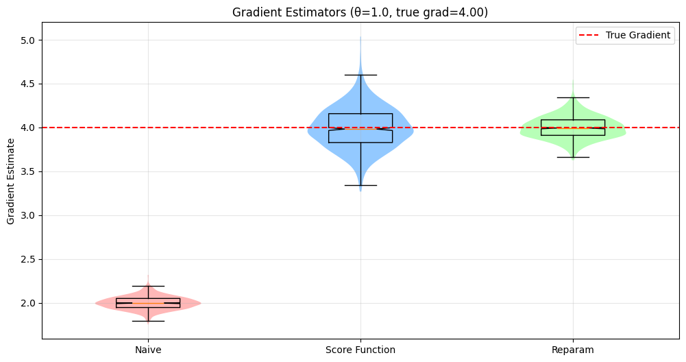
The numerical experiments coroborate our theory. The naive estimator consistently underestimates the true gradient by 2.0, though it maintains a relatively small variance. This systematic bias would make it unsuitable for optimization despite its low variance. The score function estimator corrects this bias but introduces substantial variance. While unbiased, this estimator would require many samples to achieve reliable gradient estimates. Finally, the reparameterization trick achieves a much lower variance while remaining unbiased. While this experiment is for didactic purposes only, it reproduces what is commonly found in practice: that when applicable, the reparameterization estimator tends to perform better than the score function counterpart.
Score Function Gradient Estimation in Reinforcement Learning#
Let \(G(\tau) \equiv \sum_{t=0}^T r(s_t, a_t)\) be the sum of undiscounted rewards in a trajectory \(\tau\). The stochastic optimization problem we face is to maximize:
where \(\tau = (s_0,a_0,s_1,a_1,...)\) is a trajectory and \(G(\tau)\) is the total return. Applying the score function estimator, we get:
We have eliminated the need to know the transition probabilities in this estimator since the probability of a trajectory factorizes as:
Therefore, only the policy depends on \(\boldsymbol{w}\). When taking the logarithm of this product, we get a sum where all the \(\boldsymbol{w}\)-independent terms vanish. The final estimator samples trajectories under the distribution \(p(\tau; \boldsymbol{w})\) and computes:
This is a direct application of the score function estimator. However, we rarely use this form in practice and instead make several improvements to further reduce the variance.
Leveraging Conditional Independence#
Given the Markov property of the MDP, rewards \(r_k\) for \(k < t\) are conditionally independent of action \(a_t\) given the history \(h_t = (s_0,a_0,...,s_{t-1},a_{t-1},s_t)\). This allows us to only need to consider future rewards when computing policy gradients.
The condition independence assumption means that the term \(\mathbb{E}_{\tau}\left[\sum_{t=0}^T\nabla_{\boldsymbol{w}}\log d(a_t|s_t;\boldsymbol{w})\sum_{k=0}^{t-1} r_k \right]\) vanishes. To see this, let’s factor the trajectory distribution as:
We can now re-write a single term of this summation as:
The inner expectation is zero because
The Monte Carlo estimator becomes:
The benefit of this estimator compared to the naive one is that it generally has less variance. More formally, we can show that this estimator arises from the application of a variance reduction technique known as the Extended Conditional Monte Carlo Method.
Variance Reduction via Control Variates#
A control variate is a zero-mean random variable that we subtract from our estimator to reduce variance. Given an estimator \(Z\) and a control variate \(C\) with \(\mathbb{E}[C]=0\), we can construct a new unbiased estimator:
where \(\alpha\) is a coefficient we can choose. The variance of this new estimator is:
The optimal \(\alpha\) that minimizes this variance is:
In the reinforcement learning setting, we usually choose \(C_t = \nabla_{\boldsymbol{w}}\log d(a_t|s_t;\boldsymbol{w})\) as our control variate at each timestep. For a given state \(s_t\), our estimator at time \(t\) is:
Our control variate estimator becomes:
Following the general theory, and using the fact that \(\mathbb{E}[C_t|s_t] = 0\) the optimal coefficient is:
Therefore, our variance-reduced estimator becomes:
In practice when implementing this estimator, we won’t have access to the true value function. So as we did earlier for NFQCA or SAC, we commonly learn that value function simultaneously with the policy. Do do so, we could either using a fitted value approach, or even more simply just regress from states to sum of rewards to learn what Williams 1992 called a “baseline”:
Algorithm 44 (Policy Gradient with Simple Baseline)
Input: Policy parameterization \(d(a|s;\boldsymbol{w})\), baseline function \(b(s;\boldsymbol{\theta})\)
Output: Updated policy parameters \(\boldsymbol{w}\)
Hyperparameters: Learning rates \(\alpha_w\), \(\alpha_\theta\), number of episodes \(N\), episode length \(T\)
Initialize parameters \(\boldsymbol{w}\), \(\boldsymbol{\theta}\)
For episode = 1, …, \(N\) do:
Collect trajectory \(\tau = (s_0, a_0, r_0, ..., s_T, a_T, r_T)\) using policy \(d(a|s;\boldsymbol{w})\)
Compute returns for each timestep: \(R_t = \sum_{k=t}^T r_k\)
Update baseline: \(\boldsymbol{\theta} \leftarrow \boldsymbol{\theta} + \alpha_\theta \nabla_{\boldsymbol{\theta}}\sum_{t=0}^T (R_t - b(s_t;\boldsymbol{\theta}))^2\)
For \(t = 0, ..., T\) do:
Update policy: \(\boldsymbol{w} \leftarrow \boldsymbol{w} + \alpha_w \nabla_{\boldsymbol{w}}\log d(a_t|s_t;\boldsymbol{w})(R_t - b(s_t;\boldsymbol{\theta}))\)
Return \(\boldsymbol{w}\)
When implementing this algorithm nowadays, we always using mini-batching to make full use of our GPUs. Therefore, a more representative variant for this algorithm would be:
Algorithm 45 (Policy Gradient with Optimal Control Variate and Mini-batches)
Input: Policy parameterization \(d(a|s;\boldsymbol{w})\), value function \(v(s;\boldsymbol{\theta})\)
Output: Updated policy parameters \(\boldsymbol{w}\)
Hyperparameters: Learning rates \(\alpha_w\), \(\alpha_\theta\), number of iterations \(N\), episode length \(T\), batch size \(B\), mini-batch size \(M\)
Initialize parameters \(\boldsymbol{w}\), \(\boldsymbol{\theta}\)
For iteration = 1, …, N:
Initialize empty buffer \(\mathcal{D}\)
For b = 1, …, B:
Collect trajectory \(\tau_b = (s_0, a_0, r_0, ..., s_T, a_T, r_T)\) using policy \(d(a|s;\boldsymbol{w})\)
Compute returns: \(R_t = \sum_{k=t}^T r_k\) for all t
Store tuple \((s_t, a_t, R_t)_{t=0}^T\) in \(\mathcal{D}\)
Compute value targets: \(v_{\text{target}}(s) = \frac{1}{|\mathcal{D}_s|}\sum_{(s,\cdot,R) \in \mathcal{D}_s} R\)
For value_epoch = 1, …, K:
Sample mini-batch \(\mathcal{B}_v\) of size \(M\) from \(\mathcal{D}\)
Compute value loss: \(L_v = \frac{1}{M}\sum_{(s,\cdot,R) \in \mathcal{B}_v} (v(s;\boldsymbol{\theta}) - v_{\text{target}}(s))^2\)
Update value function: \(\boldsymbol{\theta} \leftarrow \boldsymbol{\theta} - \alpha_\theta \nabla_{\boldsymbol{\theta}}L_v\)
Compute advantages: \(A(s,a) = R - v(s;\boldsymbol{\theta})\) for all \((s,a,R) \in \mathcal{D}\)
Normalize advantages: \(A \leftarrow \frac{A - \mu_A}{\sigma_A}\)
For policy_epoch = 1, …, J:
Sample mini-batch \(\mathcal{B}_\pi\) of size \(M\) from \(\mathcal{D}\)
Compute policy loss: \(L_\pi = -\frac{1}{M}\sum_{(s,a,\cdot) \in \mathcal{B}_\pi} \log d(a|s;\boldsymbol{w})A(s,a)\)
Update policy: \(\boldsymbol{w} \leftarrow \boldsymbol{w} - \alpha_w \nabla_{\boldsymbol{w}}L_\pi\)
Return \(\boldsymbol{w}\)
Generalized Advantage Estimator#
Given our control variate estimator with baseline \(v(s)\), we have:
where \(G_t\) is the return \(\sum_{k=t}^T r_k\). We can improve this estimator by considering how it relates to the advantage function, defined as:
where \(q(s_t,a_t)\) is the action-value function. Due to the Bellman equation:
This leads to the one-step TD error:
Now, let’s decompose our original term:
Expanding recursively:
GAE generalizes this by introducing a weighted version with parameter \(\lambda\):
Which simplifies to:
This formulation allows us to trade off bias and variance through \(\lambda\):
\(\lambda=0\): one-step TD error (low variance, high bias)
\(\lambda=1\): Monte Carlo estimate (high variance, low bias)
The general GAE algorithm with mini-batches is the following:
Algorithm 46 (Policy Gradient with GAE and Mini-batches)
Input: Policy parameterization \(d(a|s;\boldsymbol{w})\), value function \(v(s;\boldsymbol{\theta})\)
Output: Updated policy parameters \(\boldsymbol{w}\)
Hyperparameters: Learning rates \(\alpha_w\), \(\alpha_\theta\), number of iterations \(N\), episode length \(T\), batch size \(B\), mini-batch size \(M\), discount \(\gamma\), GAE parameter \(\lambda\)
Initialize parameters \(\boldsymbol{w}\), \(\boldsymbol{\theta}\)
For iteration = 1, …, N:
Initialize empty buffer \(\mathcal{D}\)
For b = 1, …, B:
Collect trajectory \(\tau_b = (s_0, a_0, r_0, ..., s_T, a_T, r_T)\) using policy \(d(a|s;\boldsymbol{w})\)
Compute TD errors: \(\delta_t = r_t + \gamma v(s_{t+1};\boldsymbol{\theta}) - v(s_t;\boldsymbol{\theta})\) for all t
Compute GAE advantages:
Initialize \(A_T = 0\)
For t = T-1, …, 0:
\(A_t = \delta_t + (\gamma\lambda)A_{t+1}\)
Store tuple \((s_t, a_t, A_t, v(s_t;\boldsymbol{\theta}))_{t=0}^T\) in \(\mathcal{D}\)
For value_epoch = 1, …, K:
Sample mini-batch \(\mathcal{B}_v\) of size \(M\) from \(\mathcal{D}\)
Compute value loss: \(L_v = \frac{1}{M}\sum_{(s,\cdot,\cdot,v_{\text{old}}) \in \mathcal{B}_v} (v(s;\boldsymbol{\theta}) - v_{\text{old}})^2\)
Update value function: \(\boldsymbol{\theta} \leftarrow \boldsymbol{\theta} - \alpha_\theta \nabla_{\boldsymbol{\theta}}L_v\)
Normalize advantages: \(A \leftarrow \frac{A - \mu_A}{\sigma_A}\)
For policy_epoch = 1, …, J:
Sample mini-batch \(\mathcal{B}_\pi\) of size \(M\) from \(\mathcal{D}\)
Compute policy loss: \(L_\pi = -\frac{1}{M}\sum_{(s,a,A,\cdot) \in \mathcal{B}_\pi} \log d(a|s;\boldsymbol{w})A\)
Update policy: \(\boldsymbol{w} \leftarrow \boldsymbol{w} - \alpha_w \nabla_{\boldsymbol{w}}L_\pi\)
Return \(\boldsymbol{w}\)
With \(\lambda = 0\), the GAE advantage estimator becomes just the one-step TD error:
The non-batched, purely online, GAE(0) algorithm then becomes:
Algorithm 47 (Actor-Critic with TD(0))
Input: Policy parameterization \(d(a|s;\boldsymbol{w})\), value function \(v(s;\boldsymbol{\theta})\)
Output: Updated policy parameters \(\boldsymbol{w}\)
Hyperparameters: Learning rates \(\alpha_w\), \(\alpha_\theta\), number of episodes \(N\), episode length \(T\), discount \(\gamma\)
Initialize parameters \(\boldsymbol{w}\), \(\boldsymbol{\theta}\)
For episode = 1, …, \(N\) do:
Initialize state \(s_0\)
For \(t = 0, ..., T\) do:
Sample action: \(a_t \sim d(\cdot|s_t;\boldsymbol{w})\)
Execute \(a_t\), observe \(r_t\), \(s_{t+1}\)
Compute TD error: \(\delta_t = r_t + \gamma v(s_{t+1};\boldsymbol{\theta}) - v(s_t;\boldsymbol{\theta})\)
Update value function: \(\boldsymbol{\theta} \leftarrow \boldsymbol{\theta} + \alpha_\theta \delta_t \nabla_{\boldsymbol{\theta}}v(s_t;\boldsymbol{\theta})\)
Update policy: \(\boldsymbol{w} \leftarrow \boldsymbol{w} + \alpha_w \nabla_{\boldsymbol{w}}\log d(a_t|s_t;\boldsymbol{w})\delta_t\)
Return \(\boldsymbol{w}\)
Interestingly, this version was first derived by Richard Sutton in his 1984 PhD thesis. He called it the Adaptive Heuristic Actor-Critic algorithm. As far as I know, it was not derived using the score function method outlined here, but rather through intuitive reasoning (great intuition!).
The Policy Gradient Theorem#
Sutton 1999 provided an expression for the gradient of the infinite discounted return with respect to the parameters of a parameterized policy. Here is an alternative derivation by considering a bilevel optimization problem:
subject to:
The Implicit Function Theorem states that if there is a solution to the problem \(F(\mathbf{v}, \mathbf{w}) = 0\), then we can “reparameterize” our problem as \(F(\mathbf{v}(\mathbf{w}), \mathbf{w})\) where \(\mathbf{v}(\mathbf{w})\) is an implicit function of \(\mathbf{w}\). If the Jacobian \(\frac{\partial F}{\partial \mathbf{v}}\) is invertible, then:
Here we made it clear in our notation that the derivative must be evaluated at root \((\mathbf{v}(\mathbf{w}), \mathbf{w})\) of \(F\). For the remaining of this derivation, we will drop this dependence to make notation more compact.
Applying this to our case with \(F(\mathbf{v}, \mathbf{w}) = (\mathbf{I} - \gamma \mathbf{P}_d)\mathbf{v} - \mathbf{r}_d\):
Then:
where we have defined the discounted state visitation distribution:
Remember the vector notation for MDPs:
Then taking the derivatives gives us:
Substituting back:
This is the policy gradient theorem, where \(x_\alpha(s)\) is the discounted state visitation distribution and the term in parentheses is the state-action value function \(q(s,a)\).
Normalized Discounted State Visitation Distribution#
The discounted state visitation \(x_\alpha(s)\) is not normalized. Therefore the expression we obtained above is not an expectation. However, we can tranform it into one by normalizing by \(1- \gamma\). Note that for any initial distribution \(\alpha\):
Therefore, defining the normalized state distribution \(\mu_\alpha(s) = (1-\gamma)x_\alpha(s)\), we can write:
Now we have expressed the policy gradient theorem in terms of expectations under the normalized discounted state visitation distribution. But what does sampling from \(\mu_\alpha\) means? Recall that \(\mathbf{x}_\alpha^\top = \alpha^\top(\mathbf{I} - \gamma \mathbf{P}_d)^{-1}\). Using the Neumann series expansion (valid when \(\|\gamma \mathbf{P}_d\| < 1\), which holds for \(\gamma < 1\) since \(\mathbf{P}_d\) is a stochastic matrix) we have:
We can then factor out the first term from this summation to obtain: s
The balance equation :
shows that \(\boldsymbol{\mu}_\alpha\) is a mixture distribution: with probability \(1-\gamma\) you draw a state from the initial distribution \(\alpha\) (reset), and with probability \(\gamma\) you follow the policy dynamics \(\mathbf{P}_d\) from the current state (continue). This interpretation directly connects to the geometric process: at each step you either terminate and resample from \(\alpha\) (with probability \(1-\gamma\)) or continue following the policy (with probability \(\gamma\)).
import numpy as np

def sample_from_discounted_visitation(
    alpha,
    policy,
    transition_model,
    gamma,
    n_samples=1000
):
    """Sample states from the discounted visitation distribution.

    Args:
        alpha: Initial state distribution (vector of probabilities)
        policy: Function (state -> action probabilities)
        transition_model: Function (state, action -> next state probabilities)
        gamma: Discount factor
        n_samples: Number of states to sample

    Returns:
        Array of sampled states
    """
    samples = []
    n_states = len(alpha)

    # Initialize state from alpha
    current_state = np.random.choice(n_states, p=alpha)

    for _ in range(n_samples):
        samples.append(current_state)

        # With probability (1-gamma): reset
        if np.random.random() > gamma:
            current_state = np.random.choice(n_states, p=alpha)
        # With probability gamma: continue
        else:
            # Sample action from policy
            action_probs = policy(current_state)
            action = np.random.choice(len(action_probs), p=action_probs)

            # Sample next state from transition model
            next_state_probs = transition_model(current_state, action)
            current_state = np.random.choice(n_states, p=next_state_probs)

    return np.array(samples)

# Example usage for a simple 2-state MDP
alpha = np.array([0.7, 0.3])  # Initial distribution
policy = lambda s: np.array([0.8, 0.2])  # Dummy policy
transition_model = lambda s, a: np.array([0.9, 0.1])  # Dummy transitions
gamma = 0.9

samples = sample_from_discounted_visitation(alpha, policy, transition_model, gamma)

# Check empirical distribution
print("Empirical state distribution:")
print(np.bincount(samples) / len(samples))
Empirical state distribution:
[0.857 0.143]
While the math shows that sampling from the discounted visitation distribution \(\boldsymbol{\mu}_\alpha\) would give us unbiased policy gradient estimates, Thomas (2014) demonstrated that this implementation can be detrimental to performance in practice. The issue arises because terminating trajectories early (with probability \(1-\gamma\)) reduces the effective amount of data we collect from each trajectory. This early termination weakens the learning signal, as many trajectories don’t reach meaningful terminal states or rewards.
Therefore, in practice, we typically sample complete trajectories from the undiscounted process (i.e., run the policy until natural termination or a fixed horizon) while still using \(\gamma\) in the advantage estimation. This approach preserves the full learning signal from each trajectory and has been empirically shown to lead to better performance.
This is one of several cases in RL where the theoretically optimal procedure differs from the best practical implementation.
Policy Optimization with a Model#
In this section, we’ll explore how incorporating a model of the dynamics can help us design better policy gradient estimators. Let’s begin with a pure model-free approach that uses a critic to maximize a deterministic policy:
Using the recursive structure of the Bellman equations, we can unroll our objective one step ahead:
To differentiate this objective, we need access to both a model of the dynamics and the reward function, as shown in the following expression:
While \(\boldsymbol{w}\) doesn’t appear in the outer expectation over initial states, it affects the inner expectation over next states—a distributional dependency. As a result, the product rule of calculus yields two terms: the first being an expectation, and the second being problematic for sample average estimation. However, we have tools to address this challenge: we can either apply the reparameterization trick to the dynamics or use score function estimators.
For the reparameterization approach, assuming \(s' = f(s,a,\xi;\boldsymbol{w})\) where \(\xi\) is the noise variable:
As for the score function approach:
We’ve now developed a hybrid algorithm that combines model-based and model-free approaches while integrating derivative estimators for stochastic dynamics with a deterministic policy parameterization. While this hybrid estimator remains relatively unexplored in practice, it could prove valuable for systems with specific structural properties.
Consider a robotics scenario with hybrid continuous-discrete dynamics: a robotic arm operates in continuous space but interacts with discrete object states. While the arm’s policy remains differentiable (\(\nabla_{\boldsymbol{w}} d\)), the object state transitions follow categorical distributions. In this case, reparameterization becomes impractical, but the score function approach is viable if we can compute \(\nabla_{\boldsymbol{w}} \log p(s'|s,d(s;\boldsymbol{w}))\) from the known transition model. Similar structures arise in manufacturing processes, where machine actions might be continuous and differentiable, but material state transitions often follow discrete steps with known probabilities. Note that both approaches require knowledge of transition probabilities and won’t work with pure black-box simulators or systems where we can only sample transitions without probability estimates.
Another dimension to explore in our algorithm design is the number of steps we wish to unroll our model. This allows us to better understand and control the bias-variance tradeoffs in our methods.
Backpropagation Policy Optimization#
The questions of derivative estimators only arise with stochastic dynamics. For systems with deterministic dynamics and a deterministic policy, the one-step gradient unroll simplifies to:
where \(s' = f(s,d(s;\boldsymbol{w}))\) is the deterministic next state. Notice the resemblance between this expression and that obtained for \(\nabla_{\boldsymbol{w}} J^{\text{DPMB-R}}\) above. They are essentially the same except that in the reparameterized case, the dynamics have made the dependence on the noise variable explicit and the outer expectation has been updated accordingly. This similarity arises because differentiation through reparameterized dynamics models is, in essence, backpropagation: it tracks the propagation of perturbations through a computation graph—which we refer to as a stochastic computation graph in this setting.
Still under this simplified setting with deterministic policies and dynamics, we can extend the expression for the gradient through n-steps of model unroll, leading to:
where \(s_{t+1} = f(s_t,d(s_t;\boldsymbol{w}))\) for \(t=0,\ldots,n-1\), \(s_0=s\), and \(\nabla_{\boldsymbol{w}} s_t\) follows the recursive relationship:
with base case \(\nabla_{\boldsymbol{w}} s_0 = 0\) since the initial state does not depend on the policy parameters.
At both ends of the spectrum, we have that for n=0, we fall back to the pure critic NFQCA-like approach, and for \(n=\infty\), we don’t bootstrap at all and are fully model-based without a critic. The pure model-based critic-free approach to optimization is what we may refer to as a backpropagation-based policy optimization (BPO).
But just as backpropagation through RNNs or very deep networks can be challenging due to exploding and vanishing gradients, “vanilla” Backpropagation Policy Optimization (BPO) without a critic can severely suffer from the curse of horizon. This is because it essentially implements single shooting optimization. Using a critic can be an effective remedy to this problem, allowing us to better control the bias-variance tradeoff while preserving gradient information that would be lost with a more drastic truncated backpropagation approach.
Stochastic Value Gradient (SVG)#
The stochastic value gradient framework of Heess (2015) applies the recipe for policy optimization with a model using reparameterized dynamics and action selection via randomized policies. In this setting, the stochastic policy model based reparameterized estimator over n steps is
where \(s_0 = s\) and for \(i \geq 0\), \(s_{i+1} = f(s_i,d(s_i,\epsilon_i;\boldsymbol{w}),\xi_i)\). The gradient becomes:
where \(\nabla_{\boldsymbol{w}} s_0 = 0\) and for \(i \geq 0\):
While we could implement this expression for the gradient ourselves, this approach is much easier, less error-prone, and most likely better optimized for performance when using automatic differentiation. Given a set of rollouts (for which we know the primitive noise variables), then we can compute the monte carlo objective:
where the states are generated recursively using the known noise variables: starting with initial state \(s_0^m\), each subsequent state is computed as \(s_{i+1}^m = f(s_i^m,d(s_i^m,\epsilon_i^m;\boldsymbol{w}),\xi_i^m)\). Thus, a trajectory is completely determined by just the sequence of noise variables:\((\epsilon_0^m, \xi_0^m, \epsilon_1^m, \xi_1^m, ..., \epsilon_{n-1}^m, \xi_{n-1}^m, \epsilon_n^m)\) where \(\epsilon_i^m\) are the action noise variables and \(\xi_i^m\) are the dynamics noise variables.
The choice of unroll steps \(n\) gives us precise control over the balance between model-based and critic-based components in our gradient estimator. At one extreme, setting \(n = 0\) yields a purely model-free algorithm known as SVG(0) (Heess et al., 2015), which relies entirely on the critic for value estimation:
At the other extreme, as \(n \to \infty\), we can drop the critic term (since \(\gamma^n Q \to 0\)) to obtain a purely model-based algorithm, SVG(∞):
In the 2015 paper, the authors make a specific choice to reparameterize both the dynamics and action selections using normal distributions. For the policy, they use:
where \(d(s_t;\boldsymbol{w})\) predicts the mean action and \(\sigma(s_t;\boldsymbol{w})\) predicts the standard deviation. For the dynamics:
where \(\mu(s_t,a_t;\boldsymbol{\phi})\) predicts the mean next state and \(\Sigma(s_t,a_t;\boldsymbol{\phi})\) predicts the covariance matrix.
Under this reparameterization, the n-step surrogate loss becomes:
where: $\( s_{t+1}^m(\boldsymbol{w}) = \mu(s_t^m(\boldsymbol{w}),d(s_t^m(\boldsymbol{w});\boldsymbol{w}) + \sigma(s_t^m(\boldsymbol{w});\boldsymbol{w})\epsilon_t^m;\boldsymbol{\phi}) + \Sigma(s_t^m(\boldsymbol{w}),a_t^m(\boldsymbol{w});\boldsymbol{\phi})\xi_t^m \)$
Algorithm 48 (Stochastic Value Gradients (SVG) Infinity (automatic differentiation))
Input Initial state distribution \(\rho_0(s)\), policy networks \(d(s;\boldsymbol{w})\) and \(\sigma(s;\boldsymbol{w})\), dynamics model networks \(\mu(s,a;\boldsymbol{\phi})\) and \(\Sigma(s,a;\boldsymbol{\phi})\), reward function \(r(s,a)\), rollout horizon \(T\), learning rate \(\alpha_w\), batch size \(N\)
Initialize
Policy parameters \(\boldsymbol{w}_0\) randomly
\(n \leftarrow 0\)
while not converged:
Sample batch of \(N\) initial states \(s_0^i \sim \rho_0(s)\)
Sample noise sequences \(\epsilon_{0:T}^i, \xi_{0:T}^i \sim \mathcal{N}(0,I)\) for \(i=1,\ldots,N\)
Compute objective using autodiff-enabled computation graph:
For each \(i=1,\ldots,N\):
Initialize \(s_0^i(\boldsymbol{w}) = s_0^i\)
For \(t=0\) to \(T\):
\(a_t^i(\boldsymbol{w}) = d(s_t^i(\boldsymbol{w});\boldsymbol{w}) + \sigma(s_t^i(\boldsymbol{w});\boldsymbol{w})\epsilon_t^i\)
\(s_{t+1}^i(\boldsymbol{w}) = \mu(s_t^i(\boldsymbol{w}),a_t^i(\boldsymbol{w});\boldsymbol{\phi}) + \Sigma(s_t^i(\boldsymbol{w}),a_t^i(\boldsymbol{w});\boldsymbol{\phi})\xi_t^i\)
\(J(\boldsymbol{w}) = \frac{1}{N}\sum_{i=1}^N \sum_{t=0}^T \gamma^t r(s_t^i(\boldsymbol{w}),a_t^i(\boldsymbol{w}))\)
Compute gradient using autodiff: \(\nabla_{\boldsymbol{w}}J\)
Update policy: \(\boldsymbol{w}_{n+1} \leftarrow \boldsymbol{w}_n + \alpha_w \nabla_{\boldsymbol{w}}J\)
\(n \leftarrow n + 1\)
return \(\boldsymbol{w}_n\)
Noise Inference in SVG#
The method we’ve presented so far assumes we have direct access to the noise variables \(\epsilon\) and \(\xi\) used to generate trajectories. This works well in the on-policy setting where we generate our own data. However, in off-policy scenarios where we receive externally generated trajectories, we need to infer these noise variables—a process the authors call noise inference.
For the Gaussian case discussed above, this inference is straightforward. Given an observed scalar action \(a_t\) and the current policy parameters \(\boldsymbol{w}\), we can recover the action noise \(\epsilon_t\) through inverse reparameterization:
Similarly, for the dynamics noise where states are typically vector-valued:
This simple inversion is possible because the Gaussian reparameterization is an affine transformation, which is invertible as long as \(\sigma(s_t;\boldsymbol{w})\) is non-zero for scalar actions and \(\Sigma(s_t,a_t;\boldsymbol{\phi})\) is full rank for vector-valued states. The same principle extends naturally to vector-valued actions, where \(\sigma\) would be replaced by a full covariance matrix.
More generally, this idea of invertible transformations can be extended far beyond simple Gaussian reparameterization. We could consider a sequence of invertible transformations:
where each \(f_k\) is an invertible neural network layer. The forward process can be written compactly as:
This is precisely the idea behind normalizing flows: a series of invertible transformations that can transform a simple base distribution (like a standard normal) into a complex target distribution while maintaining exact invertibility.
The noise inference in this case would involve applying the inverse transformations:
This approach offers several advantages:
More expressive policies and dynamics models capable of capturing multimodal distributions
Exact likelihood computation through the change of variables formula (can be useful for computing the log prob terms in entropy regularization for example)
Precise noise inference through the guaranteed invertibility of the flow
As far as I know, this approach has not been explored in the literature.
DPG as a Special Case of SAC#
At first glance, SAC and DPG might appear to be fundamentally different approaches to policy optimization. SAC begins with the principle of entropy maximization and policy distribution matching through KL divergence minimization, while DPG directly optimizes a deterministic policy to maximize expected Q-values. However, we can show that DPG emerges as a special case of SAC as we take the temperature parameter to zero.
Proposition 5 (Convergence of SAC to DPG)
Let \(d(\cdot|s;\boldsymbol{w}_\alpha)\) be the optimal stochastic policy for SAC with temperature \(\alpha\), and \(d(s;\boldsymbol{w}_{DPG})\) be the optimal deterministic policy gradient solution. Under appropriate assumptions, as \(\alpha \to 0\):
Assumptions:
The stochastic policy class is Gaussian with learnable mean and standard deviation:
\[ d(a|s;\boldsymbol{w}) = \mathcal{N}(\mu_w(s), \sigma_w(s)^2) \]The SAC objective for policy improvement uses the soft Q-function:
\[ \boldsymbol{w}^*_\alpha = \arg\min_w \mathbb{E}_{s\sim\rho}\left[D_{KL}\left(d(\cdot|s;\boldsymbol{w}) \| \frac{\exp(Q_{soft}(s,\cdot)/\alpha)}{\int \exp(Q_{soft}(s,b)/\alpha)db}\right)\right] \]where \(Q_{soft}\) follows the soft Bellman equation:
\[ Q_{soft}(s,a) = r(s,a) + \gamma \mathbb{E}_{s' \sim P}\left[\mathbb{E}_{a' \sim d(\cdot|s')}\left[Q_{soft}(s',a') - \alpha \log d(a'|s')\right]\right] \]The DPG objective with a deterministic policy uses the standard Q-function:
\[ \boldsymbol{w}^*_{DPG} = \arg\max_w \mathbb{E}_{s\sim\rho}\left[Q(s,d(s;\boldsymbol{w}))\right] \]where \(Q\) follows the standard Bellman equation:
\[ Q(s,a) = r(s,a) + \gamma \mathbb{E}_{s' \sim P}[Q(s',d(s';\boldsymbol{w}))] \]\(Q_{soft}(s,a)\) and \(Q(s,a)\) are continuous and achieve their maxima for each state \(s\).
Proof. At the fixed point of the soft Bellman equation, as \(\alpha \to 0\), the entropy term \(-\alpha \log d(a|s)\) vanishes, and \(Q_{soft} \to Q\). This implies that the SAC target distribution, which is proportional to \(\exp(Q_{soft}(s,a)/\alpha)\), becomes:
by Laplace’s method. The target distribution thus collapses to a delta function centered at the deterministic optimal action \(\arg\max_a Q(s,a)\).
The KL divergence term in the SAC objective measures the divergence between the stochastic policy \(d(a|s;\boldsymbol{w})\) (Gaussian) and this target distribution. For a Gaussian \(\mathcal{N}(\mu, \sigma^2)\) and a delta function \(\delta(a - a^*)\), we derive:
where \(\mathcal{N}(a^*, \epsilon^2)\) is a Gaussian approximation of the delta. Using the KL formula:
Taking the limit \(\epsilon \to 0\), the divergence diverges unless \(\mu = a^*\) and \(\sigma = 0\), where it becomes zero. Thus, minimizing the SAC objective drives \(\mu_w(s) \to \arg\max_a Q(s,a)\) and \(\sigma_w(s) \to 0\).
Consequently, the stochastic policy converges to a delta function:
Policy Optimization with a Trust Region#
Trust region methods in optimization approximate the objective function with a simpler local model within a region where we “trust” this approximation to be good. This brings about the need to define what we mean by a local region, and therefore to pick a geometry which suits our problem.
In standard optimization in the Euclidean space on \(\mathbb{R}^n\), at each iteration \(k\), we create a quadratic approximation around the current point \(x_k\):
where \(g_k = \nabla f(x_k)\) is the gradient and \(B_k\) approximates the Hessian. The trust region constrains updates using Euclidean distance:
However, when optimizing over probability distributions \(p(x;\theta)\), the Euclidean geometry becomes unnatural. Instead, the Kullback-Leibler divergence provides a more natural mean of measuring proximity:
This leads to the following trust region subproblem:
For exponential families, the KL divergence locally reduces to a quadratic form involving the Fisher Information Matrix \(I(\theta_k)\):
In both cases, after solving for the step, we evaluate the actual versus predicted reduction ratio:
This ratio determines both step acceptance and trust region adjustment:
The method accepts steps when the model prediction is sufficiently accurate: