Example COCPs

Inverted Pendulum

The inverted pendulum is a classic problem in control theory and robotics that demonstrates the challenge of stabilizing a dynamic system that is inherently unstable. The objective is to keep a pendulum balanced in the upright position by applying a control force, typically at its base. This setup is analogous to balancing a broomstick on your finger: any deviation from the vertical position will cause the system to tip over unless you actively counteract it with appropriate control actions.

We typically assume that the pendulum is mounted on a cart or movable base, which can move horizontally. The system’s state is then characterized by four variables:

1. Cart position: \( x(t) \) — the horizontal position of the base.

2. Cart velocity: \( \dot{x}(t) \) — the speed of the cart.

3. Pendulum angle: \( \theta(t) \) — the angle between the pendulum and the vertical upright position.

4. Angular velocity: \( \dot{\theta}(t) \) — the rate at which the pendulum’s angle is changing.

This setup is more complex because the controller must deal with interactions between two different types of motion: linear (the cart) and rotational (the pendulum). This system is said to be “underactuated” because the number of control inputs (one) is less than the number of state variables (four). This makes the problem more challenging and interesting from a control perspective.

We can simplify the problem by assuming that the base of the pendulum is fixed. This is akin to having the bottom of the stick attached to a fixed pivot on a table. You can’t move the base anymore; you can only apply small nudges at the pivot point to keep the stick balanced upright. In this case, you’re only focusing on adjusting the stick’s tilt without worrying about moving the base. This reduces the problem to stabilizing the pendulum’s upright orientation using only the rotational dynamics. The system’s state can now be described by just two variables:

1. Pendulum angle: \( \theta(t) \) — the angle of the pendulum from the upright vertical position.

2. Angular velocity: \( \dot{\theta}(t) \) — the rate at which the pendulum’s angle is changing.

The evolution of these two varibles is governed by the following ordinary differential equation:

(1)\[\begin{equation} \begin{bmatrix} \dot{\theta}(t) \\ \ddot{\theta}(t) \end{bmatrix} = \begin{bmatrix} \dot{\theta}(t) \\ \frac{mgl}{J_t} \sin{\theta(t)} - \frac{\gamma}{J_t} \dot{\theta}(t) + \frac{l}{J_t} u(t) \cos{\theta(t)} \end{bmatrix}, \quad y(t) = \theta(t) \end{equation}\]

where:

• \(m\) is the mass of the pendulum

• \(g\) is the acceleration due to gravity

• \(l\) is the length of the pendulum

• \(\gamma\) is the coefficient of rotational friction

• \(J_t = J + ml^2\) is the total moment of inertia, with \(J\) being the pendulum’s moment of inertia about its center of mass

• \(u(t)\) is the control force applied at the base

• \(y(t) = \theta(t)\) is the measured output (the pendulum’s angle)

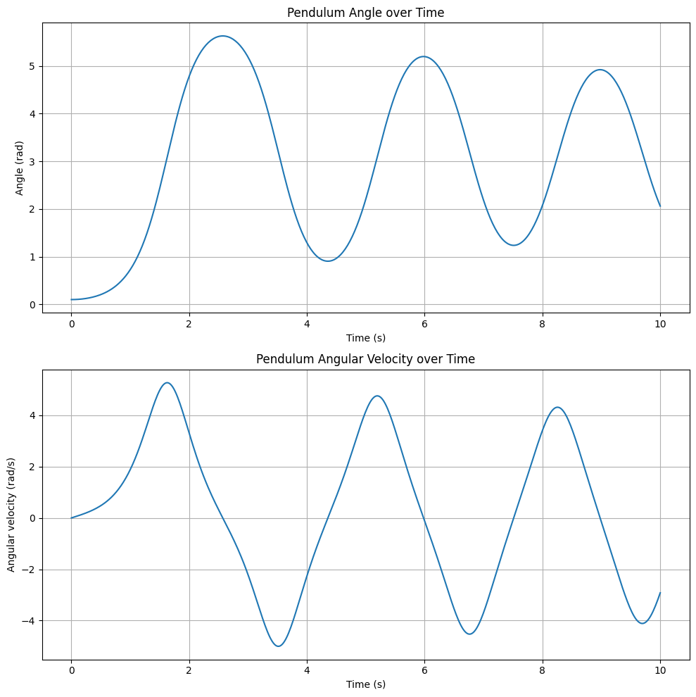
We expect that when no control is applied to the system, the rod should be falling down when started from the upright position.

Show code cell source Hide code cell source

import numpy as np
import matplotlib.pyplot as plt
from scipy.integrate import odeint
from IPython.display import HTML, display
from matplotlib.animation import FuncAnimation

# System parameters
m = 1.0  # mass of the pendulum (kg)
g = 9.81  # acceleration due to gravity (m/s^2)
l = 1.0  # length of the pendulum (m)
gamma = 0.1  # coefficient of rotational friction
J = 1/3 * m * l**2  # moment of inertia of a rod about its center of mass
J_t = J + m * l**2  # total moment of inertia

# Define the ODE for the inverted pendulum
def pendulum_ode(state, t):
    theta, omega = state
    dtheta = omega
    domega = (m*g*l/J_t) * np.sin(theta) - (gamma/J_t) * omega
    return [dtheta, domega]

# Initial conditions: slightly off vertical position
theta0 = 0.1  # initial angle (radians)
omega0 = 0  # initial angular velocity (rad/s)
y0 = [theta0, omega0]

# Time array for integration
t = np.linspace(0, 10, 500)  # Reduced number of points

# Solve ODE
solution = odeint(pendulum_ode, y0, t)

# Extract theta and omega from the solution
theta = solution[:, 0]
omega = solution[:, 1]

# Create two separate plots
fig, (ax1, ax2) = plt.subplots(2, 1, figsize=(10, 10))

# Plot for angle
ax1.plot(t, theta)
ax1.set_xlabel('Time (s)')
ax1.set_ylabel('Angle (rad)')
ax1.set_title('Pendulum Angle over Time')
ax1.grid(True)

# Plot for angular velocity
ax2.plot(t, omega)
ax2.set_xlabel('Time (s)')
ax2.set_ylabel('Angular velocity (rad/s)')
ax2.set_title('Pendulum Angular Velocity over Time')
ax2.grid(True)

plt.tight_layout()
plt.show()

# Function to create animation frames
def get_pendulum_position(theta):
    x = l * np.sin(theta)
    y = l * np.cos(theta)
    return x, y

# Create animation
fig, ax = plt.subplots(figsize=(8, 8))
line, = ax.plot([], [], 'o-', lw=2)
time_text = ax.text(0.02, 0.95, '', transform=ax.transAxes)

def init():
    ax.set_xlim(-1.2*l, 1.2*l)
    ax.set_ylim(-1.2*l, 1.2*l)  # Adjusted to show full range of motion
    ax.set_aspect('equal', adjustable='box')
    return line, time_text

def animate(i):
    x, y = get_pendulum_position(theta[i])
    line.set_data([0, x], [0, y])
    time_text.set_text(f'Time: {t[i]:.2f} s')
    return line, time_text

anim = FuncAnimation(fig, animate, init_func=init, frames=len(t), interval=40, blit=True)
plt.title('Inverted Pendulum Animation')
ax.grid(True)

# Convert animation to JavaScript
js_anim = anim.to_jshtml()

# Close the figure to prevent it from being displayed
plt.close(fig)

# Display only the JavaScript animation
display(HTML(js_anim))

Once Loop Reflect

Pendulum in the Gym Environment

Let’s examine the code and reverse-engineer the original continuous-time problem hidden behind the abstraction layer. Although the pendulum problem may have limited practical relevance as a real-world application, it serves as an excellent example for our analysis. In the current version of Pendulum, we find that the Gym implementation uses a simplified model. Like our implementation, it assumes a fixed base and doesn’t model cart movement. The state is also represented by the pendulum angle and angular velocity. However, the equations of motion implemented in the Gym environment are different and correspond to the following ODE:

\[\begin{align*} \dot{\theta} &= \theta_{dot} \\ \dot{\theta}_{dot} &= \frac{3g}{2l} \sin(\theta) + \frac{3}{ml^2} u \end{align*}\]

Compared to our simplified model, the Gym implementation makes the following additional assumptions:

1. It omits the term \(\frac{\gamma}{J_t} \dot{\theta}(t)\), which represents damping or air resistance. This means that it assumes an idealized pendulum that doesn’t naturally slow down over time.

2. It uses \(ml^2\) instead of \(J_t = J + ml^2\), which assumes that all mass is concentrated at the pendulum’s end (like a point mass on a massless rod), rather than accounting for mass distribution along the pendulum.

3. The control input \(u\) is applied directly, without a \(\cos \theta(t)\) term, which means that the applied torque has the same effect regardless of the pendulum’s position, rather than varying with angle. For example, imagine trying to push a door open. When the door is almost closed (pendulum near vertical), a small push perpendicular to the door (analogous to our control input) can easily start it moving. However, when the door is already wide open (pendulum horizontal), the same push has little effect on the door’s angle. In a more detailed model, this would be captured by the \(\cos \theta(t)\) term, which is maximum when the pendulum is vertical (\(\cos 0° = 1\)) and zero when horizontal (\(\cos 90° = 0\)).

The goal remains to stabilize the rod upright, but the way in which this encoded is through the following instantenous cost function:

\[\begin{align*} c(\theta, \dot{\theta}, u) &= (\text{normalize}(\theta))^2 + 0.1\dot{\theta}^2 + 0.001u^2\\ \text{normalize}(\theta) &= ((\theta + \pi) \bmod 2\pi) - \pi \end{align*}\]

This cost function penalizes deviations from the upright position (first term), discouraging rapid motion (second term), and limiting control effort (third term). The relative weights has been manually chosen to balance the primary goal of upright stabilization with the secondary aims of smooth motion and energy efficiency. The normalization ensures that the angle is always in the range \([-\pi, \pi]\) so that the pendulum positions (e.g., \(0\) and \(2\pi\)) are treated identically, which could otherwise confuse learning algorithms.

Studying the code further, we find that it imposes bound constraints on both the control input and the angular velocity through clipping operations:

\[\begin{align*} u &= \max(\min(u, u_{max}), -u_{max}) \\ \dot{\theta} &= \max(\min(\dot{\theta}, \dot{\theta}_{max}), -\dot{\theta}_{max}) \end{align*}\]

Where \(u_{max} = 2.0\) and \(\dot{\theta}_{max} = 8.0\). Finally, when inspecting the step function, we find that the dynamics are discretized using forward Euler under a fixed step size of \(h=0.0.5\). Overall, the discrete-time trajectory optimization problem implemented in Gym is the following:

\[\begin{align*} \min_{u_k} \quad & J = \sum_{k=0}^{N-1} c(\theta_k, \dot{\theta}_k, u_k) \\ \text{subject to:} \quad & \theta_{k+1} = \theta_k + \dot{\theta}_k \cdot h \\ & \dot{\theta}_{k+1} = \dot{\theta}_k + \left(\frac{3g}{2l}\sin(\theta_k) + \frac{3}{ml^2}u_k\right) \cdot h \\ & -u_{\max} \leq u_k \leq u_{\max} \\ & -\dot{\theta}_{\max} \leq \dot{\theta}_k \leq \dot{\theta}_{\max}, \quad k = 0, 1, ..., N-1 \\ \text{given:} \quad & \theta_0 = \theta_{\text{initial}}, \quad \dot{\theta}_0 = \dot{\theta}_{\text{initial}}, \quad N = 200 \end{align*}\]

with \(g = 10.0\), \(l = 1.0\), \(m = 1.0\), \(u_{max} = 2.0\), and \(\dot{\theta}_{max} = 8.0\). This discrete-time problem corresponds to the following continuous-time optimal control problem:

\[\begin{align*} \min_{u(t)} \quad & J = \int_{0}^{T} c(\theta(t), \dot{\theta}(t), u(t)) dt \\ \text{subject to:} \quad & \dot{\theta}(t) = \dot{\theta}(t) \\ & \ddot{\theta}(t) = \frac{3g}{2l}\sin(\theta(t)) + \frac{3}{ml^2}u(t) \\ & -u_{\max} \leq u(t) \leq u_{\max} \\ & -\dot{\theta}_{\max} \leq \dot{\theta}(t) \leq \dot{\theta}_{\max} \\ \text{given:} \quad & \theta(0) = \theta_0, \quad \dot{\theta}(0) = \dot{\theta}_0, \quad T = 10 \text{ seconds} \end{align*}\]

Heat Exchanger

We are considering a system where fluid flows through a tube, and the goal is to control the temperature of the fluid by adjusting the temperature of the tube’s wall over time. The wall temperature, denoted as \( T_w(t) \), can be changed as a function of time, but it remains the same along the length of the tube. On the other hand, the temperature of the fluid inside the tube, \( T(z, t) \), depends both on its position along the tube \( z \) and on time \( t \). It evolves according to the following partial differential equation:

\[ \frac{\partial T}{\partial t} = -v \frac{\partial T}{\partial z} + \frac{h}{\rho C_p} (T_w(t) - T) \]

where we have:

• \( v \): the average speed of the fluid moving through the tube,

• \( h \): how easily heat transfers from the wall to the fluid,

• \( \rho \) and \( C_p \): the fluid’s density and heat capacity.

This equation describes how the fluid’s temperature changes as it moves along the tube and interacts with the tube’s wall temperature. The fluid enters the tube with an initial temperature \( T_0 \) at the inlet (where \( z = 0 \)). Our objective is to adjust the wall temperature \( T_w(t) \) so that by a specific final time \( t_f \), the fluid’s temperature reaches a desired distribution \( T_s(z) \) along the length of the tube. The relationship for \( T_s(z) \) under steady-state conditions (ie. when changes over time are no longer considered), is given by:

\[ \frac{d T_s}{d z} = \frac{h}{v \rho C_p}[\theta - T_s] \]

where \( \theta \) is a constant temperature we want to maintain at the wall. The objective is to control the wall temperature \( T_w(t) \) so that by the end of the time interval \( t_f \), the fluid temperature \( T(z, t_f) \) is as close as possible to the desired distribution \( T_s(z) \). This can be formalized by minimizing the following quantity:

\[ I = \int_0^L \left[T(z, t_f) - T_s(z)\right]^2 dz \]

where \( L \) is the length of the tube. Additionally, we require that the wall temperature cannot exceed a maximum allowable value \( T_{\max} \):

\[ T_w(t) \leq T_{\max} \]

Nuclear Reactor

In a nuclear reactor, neutrons interact with fissile nuclei, causing nuclear fission. This process produces more neutrons and smaller fissile nuclei called precursors. The precursors subsequently absorb more neutrons, generating “delayed” neutrons. The kinetic energy of these products is converted into thermal energy through collisions with neighboring atoms. The reactor’s power output is determined by the concentration of neutrons available for nuclear fission.

The reaction kinetics can be modeled using a system of ordinary differential equations:

\[\begin{align*} \dot{x}(t) &= \frac{r(t)x(t) - \alpha x^2(t) - \beta x(t)}{\tau} + \mu y(t), & x(0) &= x_0 \\ \dot{y}(t) &= \frac{\beta x(t)}{\tau} - \mu y(t), & y(0) &= y_0 \end{align*}\]

where:

• \(x(t)\): concentration of neutrons at time \(t\)

• \(y(t)\): concentration of precursors at time \(t\)

• \(t\): time

• \(r(t) = r[u(t)]\): degree of change in neutron multiplication at time \(t\) as a function of control rod displacement \(u(t)\)

• \(\alpha\): reactivity coefficient

• \(\beta\): fraction of delayed neutrons

• \(\mu\): decay constant for precursors

• \(\tau\): average time taken by a neutron to produce a neutron or precursor

The power output can be adjusted based on demand by inserting or retracting a neutron-absorbing control rod. Inserting the control rod absorbs neutrons, reducing the heat flux and power output, while retracting the rod has the opposite effect.

The objective is to change the neutron concentration \(x(t)\) from an initial value \(x_0\) to a stable value \(x_\mathrm{f}\) at time \(t_\mathrm{f}\) while minimizing the displacement of the control rod. This can be formulated as an optimal control problem, where the goal is to find the control function \(u(t)\) that minimizes the objective functional:

\[\begin{equation*} I = \int_0^{t_\mathrm{f}} u^2(t) \, \mathrm{d}t \end{equation*}\]

subject to the final conditions:

\[\begin{align*} x(t_\mathrm{f}) &= x_\mathrm{f} \\ \dot{x}(t_\mathrm{f}) &= 0 \end{align*}\]

and the constraint \(|u(t)| \leq u_\mathrm{max}\)

Chemotherapy

Chemotherapy uses drugs to kill cancer cells. However, these drugs can also have toxic effects on healthy cells in the body. To optimize the effectiveness of chemotherapy while minimizing its side effects, we can formulate an optimal control problem.

The drug concentration \(y_1(t)\) and the number of immune cells \(y_2(t)\), healthy cells \(y_3(t)\), and cancer cells \(y_4(t)\) in an organ at any time \(t\) during chemotherapy can be modeled using a system of ordinary differential equations:

\[\begin{align*} \dot{y}_1(t) &= u(t) - \gamma_6 y_1(t) \\ \dot{y}_2(t) &= \dot{y}_{2,\text{in}} + r_2 \frac{y_2(t) y_4(t)}{\beta_2 + y_4(t)} - \gamma_3 y_2(t) y_4(t) - \gamma_4 y_2(t) - \alpha_2 y_2(t) \left(1 - e^{-y_1(t) \lambda_2}\right) \\ \dot{y}_3(t) &= r_3 y_3(t) \left(1 - \beta_3 y_3(t)\right) - \gamma_5 y_3(t) y_4(t) - \alpha_3 y_3(t) \left(1 - e^{-y_1(t) \lambda_3}\right) \\ \dot{y}_4(t) &= r_1 y_4(t) \left(1 - \beta_1 y_4(t)\right) - \gamma_1 y_3(t) y_4(t) - \gamma_2 y_2(t) y_4(t) - \alpha_1 y_4(t) \left(1 - e^{-y_1(t) \lambda_1}\right) \end{align*}\]

where:

• \(y_1(t)\): drug concentration in the organ at time \(t\)

• \(y_2(t)\): number of immune cells in the organ at time \(t\)

• \(y_3(t)\): number of healthy cells in the organ at time \(t\)

• \(y_4(t)\): number of cancer cells in the organ at time \(t\)

• \(\dot{y}_{2,\text{in}}\): constant rate of immune cells entering the organ to fight cancer cells

• \(u(t)\): rate of drug injection into the organ at time \(t\)

• \(r_i, \beta_i\): constants in the growth terms

• \(\alpha_i, \lambda_i\): constants in the decay terms due to the action of the drug

• \(\gamma_i\): constants in the remaining decay terms

The objective is to minimize the number of cancer cells \(y_4(t)\) in a specified time \(t_\mathrm{f}\) while using the minimum amount of drug to reduce its toxic effects. This can be formulated as an optimal control problem, where the goal is to find the control function \(u(t)\) that minimizes the objective functional:

\[\begin{equation*} I = y_4(t_\mathrm{f}) + \int_0^{t_\mathrm{f}} u(t) \, \mathrm{d}t \end{equation*}\]

subject to the system dynamics, initial conditions, and the constraint \(u(t) \geq 0\).

Additional constraints may include:

• Maintaining a minimum number of healthy cells during treatment:

  \[\begin{equation*} y_3(t) \geq y_{3,\min} \end{equation*}\]

• Imposing an upper limit on the drug dosage:

  \[\begin{equation*} u(t) \leq u_\max \end{equation*}\]

Government Corruption

In this model from Feichtinger and Wirl (1994), we aim to understand the incentives for politicians to engage in corrupt activities or to combat corruption. The model considers a politician’s popularity as a dynamic process that is influenced by the public’s memory of recent and past corruption. The objective is to find conditions under which self-interested politicians would choose to be honest or dishonest.

The model introduces the following notation:

• \(C(t)\): accumulated awareness (knowledge) of past corruption at time \(t\)

• \(u(t)\): extent of corruption (politician’s control variable) at time \(t\)

• \(\delta\): rate of forgetting past corruption

• \(P(t)\): politician’s popularity at time \(t\)

• \(g(P)\): growth function of popularity; \(g''(P) < 0\)

• \(f(C)\): function measuring the loss of popularity caused by \(C\); \(f'(C) > 0\), \(f''(C) \geq 0\)

• \(U_1(P)\): benefits associated with being popular; \(U_1'(P) > 0\), \(U_1''(P) \leq 0\)

• \(U_2(u)\): benefits resulting from bribery and fraud; \(U_2'(u) > 0\), \(U_2''(u) < 0\)

• \(r\): discount rate

The dynamics of the public’s memory of recent and past corruption \(C(t)\) are modeled as:

\[\begin{align*} \dot{C}(t) &= u(t) - \delta C(t), \quad C(0) = C_0 \end{align*}\]

The evolution of the politician’s popularity \(P(t)\) is governed by:

\[\begin{align*} \dot{P}(t) &= g(P(t)) - f(C(t)), \quad P(0) = P_0 \end{align*}\]

The politician’s objective is to maximize the following objective:

\[\begin{equation*} \int_0^{\infty} e^{-rt} [U_1(P(t)) + U_2(u(t))] \, \mathrm{d}t \end{equation*}\]

subject to the dynamics of corruption awareness and popularity.

The optimal control problem can be formulated as follows:

\[\begin{align*} \max_{u(\cdot)} \quad & \int_0^{\infty} e^{-rt} [U_1(P(t)) + U_2(u(t))] \, \mathrm{d}t \\ \text{s.t.} \quad & \dot{C}(t) = u(t) - \delta C(t), \quad C(0) = C_0 \\ & \dot{P}(t) = g(P(t)) - f(C(t)), \quad P(0) = P_0 \end{align*}\]

The state variables are the accumulated awareness of past corruption \(C(t)\) and the politician’s popularity \(P(t)\). The control variable is the extent of corruption \(u(t)\). The objective functional represents the discounted stream of benefits coming from being honest (popularity) and from being dishonest (corruption).