Trajectory Optimization in Continuous Time#
As in the discrete-time setting, we work with three continuous-time variants that differ only in how the objective is written while sharing the same dynamics, path constraints, and bounds. The path constraints \(\mathbf{g}(\mathbf{x}(t),\mathbf{u}(t))\le \mathbf{0}\) are pointwise in time, and the bounds \(\mathbf{x}_{\min}\le \mathbf{x}(t)\le \mathbf{x}_{\max}\) and \(\mathbf{u}_{\min}\le \mathbf{u}(t)\le \mathbf{u}_{\max}\) are understood in the same pointwise sense.
Definition 1 (Mayer Problem)
Definition 2 (Lagrange Problem)
Definition 3 (Bolza Problem)
These three forms are different lenses on the same task. Bolza contains both terminal and running terms. Lagrange can be turned into Mayer by augmenting the state with an accumulator:
with the original dynamics left unchanged. Mayer is a special case of Bolza with zero running cost. We will use these equivalences freely, since a numerical method cares only about what must be evaluated and where those evaluations are taken.
With this catalog in place, we now pass from functions to finite representations.
Direct Transcription Methods#
The discrete-time problems of the previous chapter already suggested how to proceed: we convert a continuous problem into one over finitely many numbers by deciding where to look at the trajectories and how to interpolate between those looks. We place a mesh \(t_0<t_1<\cdots<t_N=t_f\) and, inside each window \([t_k,t_{k+1}]\), select a small set of interior fractions \(\{\tau_j\}\) on the reference interval \([0,1]\). The running cost is additive over windows, so we write it as a sum of local integrals, map each window to \([0,1]\), and approximate each local integral by a quadrature rule with nodes \(\tau_j\) and weights \(w_j\). This produces
with \(h_k=t_{k+1}-t_k\). The dynamics are treated in the same way by the fundamental theorem of calculus,
so the places where we “pay” running cost are the same places where we “account” for state changes. Path constraints and bounds are then enforced at the same interior times. In the infinite-horizon discounted case, the same formulas apply with an extra factor \(e^{-\rho(t_k+h_k\tau_j)}\) multiplying the weights in the cost.
The values \(\mathbf{x}(t_k+h_k\tau_j)\) and \(\mathbf{u}(t_k+h_k\tau_j)\) do not exist a priori. We create them by a finite representation. One option is shooting: parameterize \(\mathbf{u}\) on the mesh, integrate the ODE across each window with a chosen numerical step, and read interior values from that step. Another is collocation: represent \(\mathbf{x}\) inside each window by a local polynomial and choose its coefficients so that the ODE holds at the interior nodes. Both constructions lead to the same structure: a nonlinear program whose objective is a composite quadrature of the running term (plus any terminal term in the Bolza case) and whose constraints are algebraic relations that encode the ODE and the pointwise inequalities at the selected nodes.
Specific choices recover familiar schemes. If we use the left endpoint as the single interior node, we obtain the forward Euler transcription. If we use both endpoints with equal weights, we obtain the trapezoidal transcription. Higher-order rules arise when we include interior nodes and richer polynomials for \(\mathbf{x}\). What matters here is the unifying picture: choose nodes, translate integrals into weighted sums, and couple those evaluations to a finite trajectory representation so that cost and physics are enforced at the same places. This is the organizing idea that will guide the rest of the chapter.
Discretizing cost and dynamics together#
In a continuous-time OCP, integrals appear twice: in the objective, which accumulates running cost over time, and implicitly in the dynamics, since state changes over any interval are the integral of the vector field. To compute, we must approximate both the integrals and the unknown functions \(\mathbf{x}(t)\) and \(\mathbf{u}(t)\) with finitely many numbers that an optimizer can manipulate.
A natural way to do this is to lay down a finite set of time points (a mesh) over the horizon. You can think of the mesh as a grid we overlay on the “true” trajectories that exist as mathematical objects but are not directly accessible. Our aim is to approximate those trajectories and their integrals using values and simple models tied to the mesh. Using the same mesh for both the cost and the dynamics keeps the representation coherent: we evaluate what we pay and how the state changes at consistent times.
Concretely, we begin by choosing a mesh
The running cost is additive over disjoint intervals. When the horizon \([t_0,t_f]\) is partitioned by the mesh, additivity (linearity) of the integral gives
This identity is exact: it is just the additivity (linearity) of the Lebesgue/Riemann integral over a partition. No approximation has been made yet. Approximations enter only when we later replace each window integral by a quadrature rule: a finite set of nodes and positive weights prescribing an integral approximation. This sets the table for three important ingredients that we will use throughout the chapter.
First, it turns a global object into local contributions that live on each \([t_k,t_{k+1}]\). Numerical integration is most effective when it is composite: we approximate each small interval integral and then sum the results. Doing so controls error uniformly, because the global quadrature error is the accumulation of local errors that shrink with the step size. It also allows non-uniform steps \(h_k=t_{k+1}-t_k\), which we will use later for mesh refinement.
Second, the split aligns the cost with the local dynamics constraints. On each interval the ODE can be written, by the fundamental theorem of calculus, as
When we approximate this integral, we introduce interior evaluation points \(t_{k,j}\in[t_k,t_{k+1}]\). Using the same points in the cost and in the dynamics ties \(\mathbf{x}\) and \(\mathbf{u}\) together coherently: the places where we “pay” for running cost are also the places where we enforce the ODE. This avoids a mismatch between where we approximate the objective and where we impose feasibility.
Third, the decomposition yields a nonlinear program with sparse structure. Each interval contributes a small block to the objective and constraints that depends only on variables from that interval (and its endpoints). Modern solvers exploit this banded sparsity to scale to long horizons.
With the split justified, we standardize the approximation. Map each interval to a reference domain via \(t=t_k+h_k\tau\) with \(\tau\in[0,1]\) and \(dt=h_k\,d\tau\). A quadrature rule on \([0,1]\) is specified by evaluation points \(\{\tau_j\}_{j=1}^q \subset [0,1]\) and positive weights \(\{w_j\}_{j=1}^q\) such that, for a smooth \(\phi\),
Applying it on each interval gives
Summing these window contributions gives a composite approximation of the integral over \([t_0,t_f]\):
The outer index \(k\) indicates the window; the inner index \(i\) indicates the samples within that window; the factor \(h_k\) appears from the change of variables.
The dynamics admit the same treatment. By the fundamental theorem of calculus,
Replacing this integral by a quadrature rule that uses the same nodes produces the window defect relation
where \(\{b_j\}\) are the weights used for the ODE. Path constraints \(\mathbf{g}(\mathbf{x}(t),\mathbf{u}(t))\le 0\) are imposed at selected nodes \(t_{k,j}\) in the same spirit. Using the same evaluation points for cost and dynamics keeps the representation coherent: we “pay” running cost and “account” for state changes at the same times.
On the choice of interior points#
Once we select a mesh \(t_0<\cdots<t_N\) and interior fractions \(\{\tau_j\}_{j=1}^q\) per window \([t_k,t_{k+1}]\), we need \(\mathbf{x}(t_{k,j})\) and \(\mathbf{u}(t_{k,j})\) at the evaluation times \(t_{k,j} := t_k + h_k\tau_j\). These values do not preexist. They come from one of two constructions that align with the standard quadrature taxonomy: step-function based and interpolating-function based rules.
Step-function based construction (piecewise constants; rectangle or midpoint)#
Here we approximate the relevant time functions by step functions on each window. For controls, a common choice is piecewise-constant:
For the running cost and the vector field, the corresponding quadrature is a rectangle rule on \([t_k,t_{k+1}]\). Using the left endpoint gives
and replacing the dynamics integral by the same step-function idea yields the forward Euler relation
If we prefer the midpoint rectangle rule, we sample at \(t_{k+\frac12}=t_k+\tfrac{h_k}{2}\). In practice we then generate \(\mathbf{x}_{k+\frac12}\) by a half-step of the chosen integrator, and set \(\mathbf{u}_{k+\frac12}=\mathbf{u}_k\) (piecewise-constant) or an average if we allow a short linear segment. Either way, interior values come from integrating forward given a step-function model for \(\mathbf{u}\) and a rectangle-rule view of the integrals. This is the shooting viewpoint. Single shooting keeps only control parameters as decision variables; multiple shooting adds the window-start states and enforces step consistency.
Interpolating-function based construction (low-order polynomials; trapezoid, Simpson, Gauss/Radau/Lobatto)#
Here we approximate time functions by polynomials on each window. If we interpolate \(\mathbf{x}(t)\) linearly between endpoints, the cost naturally uses the trapezoidal rule
and the dynamics use the matched trapezoidal defect
With a quadratic interpolation that includes the midpoint, Simpson’s rule appears in the cost and the Hermite–Simpson relations tie \(\mathbf{x}_{k+\frac12}\) to endpoint values and slopes. More generally, collocation chooses interior nodes on \([t_k,t_{k+1}]\) (equally spaced gives Newton–Cotes like trapezoid or Simpson; Gaussian points give Gauss, Radau, or Lobatto schemes) and enforces the ODE at those nodes:
with continuity at endpoints. The interior values \(\mathbf{x}(t_{k,j})\) are evaluations of the decision polynomials; \(\mathbf{u}(t_{k,j})\) follows from the chosen control interpolation (constant, linear, or quadratic). The running cost is evaluated by the same interpolatory quadrature at the same nodes, which keeps “where we pay” aligned with “where we enforce.”
Polynomial Interpolation#
We often want to construct a function that passes through a given set of points. For example, suppose we know a function should satisfy:
These are called interpolation constraints. Our goal is to find a function \(f(x)\) that satisfies all of them exactly.
To make the problem tractable, we restrict ourselves to a class of functions. In polynomial interpolation, we assume that \(f(x)\) is a polynomial of degree at most \(N\). That means we are trying to find coefficients \(c_0, \dots, c_N\) such that
where the functions \(\phi_n(x)\) form a basis for the space of polynomials. The most common choice is the monomial basis, where \(\phi_n(x) = x^n\). This gives:
Other valid bases include Legendre, Chebyshev, and Lagrange polynomials, each chosen for specific numerical properties. But all span the same function space.
To find a unique solution, we need the number of unknowns (the \(c_n\)) to match the number of constraints. Since a degree-\(N\) polynomial has \(N+1\) coefficients, we need:
So if we want a function that passes through 4 points, we need a cubic polynomial (\(N = 3\)). Choosing a higher degree than necessary would give us infinitely many solutions; a lower degree may make the problem unsolvable.
Solving for the Coefficients (Monomial Basis)#
If we fix the basis functions to be monomials, we can build a system of equations by plugging in each \(x_i\) into \(f(x)\). This gives:
This system can be written in matrix form as:
The matrix on the left is called the Vandermonde matrix. Solving this system gives the coefficients \(c_n\) that define the interpolating polynomial.
Using a Different Basis#
We don’t have to use monomials. We can pick any set of basis functions \(\phi_n(x)\), such as Chebyshev or Fourier modes, and follow the same steps. The interpolating function becomes:
and each interpolation constraint becomes:
Assembling these into a system gives:
From here, we solve as before and reconstruct \(f(x)\).
Derivative Constraints#
Sometimes, instead of a value constraint \(f(x_i) = y_i\), we want to impose a slope constraint \(f'(x_i) = s_i\). This is common in applications like spline interpolation or collocation methods, where derivative information is available from an ODE.
Since
we can directly write the slope constraint:
To enforce this, we replace one of the interpolation equations in our system with this slope constraint. The resulting system still has \(m+1\) equations and \(N+1 = m+1\) unknowns.
Concretely, suppose we have \(k+1\) value constraints at nodes \(X=\{x_0,\ldots,x_k\}\) with values \(Y=\{y_0,\ldots,y_k\}\) and \(r\) slope constraints at nodes \(Z=\{z_1,\ldots,z_r\}\) with slopes \(S=\{s_1,\ldots,s_r\}\), with \(k+1+r=N+1\). The linear system for the coefficients \(\mathbf{c}=[c_0,\ldots,c_N]^\top\) is
If a value and a slope are imposed at the same node, take \(z_j=x_i\) and include both the value row and the derivative row; the system remains square. In the monomial basis, the top block is the Vandermonde matrix and the derivative block has entries \(n\,x^{\,n-1}\). Once solved for \(\mathbf{c}\), reconstruct
Interpolating ODE Trajectories (Collocation)#
Having established the general framework of interpolation, we now apply these concepts to the specific context of approximating trajectories governed by ordinary differential equations. The idea of applying polynomial interpolation with derivative constraints yields a method known as “collocation”. More precisely, a degree-\(s\) collocation method is a way to discretize an ordinary differential equation (ODE) by approximating the solution on each time interval with a polynomial of degree \(s\), and then enforcing that this polynomial satisfies the ODE exactly at \(s\) carefully chosen points (the collocation nodes).
Consider a dynamical system described by the ordinary differential equation:
where \(\mathbf{x}(t)\) represents the state trajectory and \(\mathbf{u}(t)\) denotes the control input. Let us focus on a single mesh interval \([t_k,t_{k+1}]\) with step size \(h_k := t_{k+1}-t_k\). To work with a standardized domain, we introduce the transformation \(t = t_k + h_k\tau\) that maps the physical interval \([t_k,t_{k+1}]\) to the reference interval \([0,1]\). On this reference interval, we select a set of collocation nodes \(\{\tau_j\}_{j=0}^K \subset [0,1]\).
Our goal is now to approximate the unknown trajectory using a polynomial of degree \(K\). Using a monomial basis, we represent (parameterize) our trajectory as:
where \(\mathbf{a}_n \in \mathbb{R}^d\) are coefficient vectors to be determined. Collocation enforces the differential equation at a chosen set of nodes on \([0,1]\). Depending on the node family, these nodes may be interior-only or may include one or both endpoints. With the polynomial state model, we can differentiate analytically. Using the change of variables \(t=t_k+h_k\,\tau\), we obtain:
The collocation condition requires that this polynomial derivative equals the right-hand side of the ODE at each collocation node \(\tau_j\):
where \(\mathbf{u}_j\) represents the control value at node \(\tau_j\).
Boundary Conditions and Node Families#
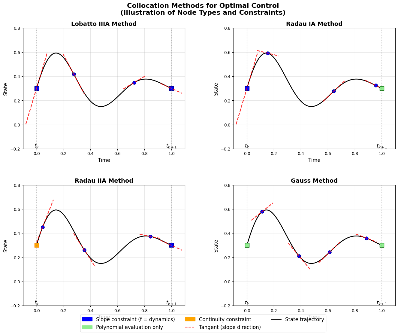
Fig. 1 Collocation node families and where slope and continuity constraints are enforced.#
The choice of collocation nodes determines how boundary conditions are handled and affects the resulting discretization properties. Three standard families are commonly used: Labatto, Randau and and Gauss.
Let’s consider these three setup with more generality over any given basis. We start again by taking a mesh interval \([t_k,t_{k+1}]\) of length \(h_k=t_{k+1}-t_k\) and reparametrize time by
We then choose to represent the (unknown) state by a degree–\(K\) polynomial
where \(\{\phi_n\}_{n=0}^K\) is any linearly independent basis of polynomials of degree \(\le K\), and \(\mathbf{a}_0,\dots,\mathbf{a}_K\) are vector coefficients to be determined.
The collocation condition mean that we require for the chosen \(K\) collocation points that: $\( \frac{d}{dt}\mathbf{x}_h\bigl(\tau_j\bigr) \;=\; \mathbf{f}\bigl(\mathbf{x}_h(\tau_j),\mathbf{u}_h(\tau_j),t_k+h_k\tau_j\bigr), \qquad j=0,1,\dots,K, \)$
which, using \(\tfrac{d}{dt}=(1/h_k)\tfrac{d}{d\tau}\), becomes
Put simply: choose some nodes inside the interval, and at each of those nodes force the slope of the polynomial approximation to match the slope prescribed by the ODE. What we mean by the expression “collocation conditions” is simply to say that we want to satisfy a set of “slope-matching equations” at the chosen nodes.
By definition of the mesh variables,
and (if you sample the control at endpoints)
With the monomial basis,
For the derivative, \(\phi_n'(\tau)=n\,\tau^{n-1}\), so
When chaining intervals into a global trajectory, direct collocation enforces state continuity by construction: the variable \(\mathbf{x}_{k+1}\) at the end of one interval is the same as the starting variable of the next. What is not enforced automatically is slope continuity; the derivative at the end of one interval generally does not match the derivative at the start of the next. Different collocation methods may have different slope continuity properties depending on the chosen collocation nodes.
Lobatto Nodes (endpoints included):
The family of Labotto methods correspond to any set of so-called Lobatto nodes \(\{\tau_j\}_{j=0}^K\) with the specificity that we require \(\tau_0=0\) and \(\tau_K=1\). Let’s assume that we work with the power (monomial) basis \(\phi_n(\tau)=\tau^n\), so that
Differentiating \(\mathbf{x}_h\) with respect to \(\tau\) gives
Since we have the chain rule \(\frac{d}{dt} = \frac{1}{h_k}\frac{d}{d\tau}\) from the time transformation \(t = t_k + h_k\tau\), the time derivative becomes
so the collocation equations at Lobatto nodes are
For \(j=0\) and \(j=K\), these conditions become:
With the monomial basis \(\phi_n(\tau)=\tau^n\), we have \(\phi_n'(0)=n\delta_{n,1}\) (only \(\phi_1'=1\), others vanish) and \(\phi_n'(1)=n\). Also, \(\phi_n(0)=\delta_{n,0}\) and \(\phi_n(1)=1\) for all \(n\). This simplifies the endpoint conditions to:
These equations enforce that the polynomial’s slope at both endpoints matches the ODE’s prescribed slope, which is why the figure shows red tangent lines at both endpoints for Lobatto methods.
Radau Nodes (one endpoint included): Radau points include only one endpoint. Radau-I includes the left endpoint (\(\tau_0 = 0\)) while Radau-II includes the right endpoint (\(\tau_K = 1\)). This means that a radau collocation is defined by any set of collocation nodes such that \(\tau_K = 1\). This translates into requireing that we match the ODE over the mesh only at the right endpoiunt in addition to the interior nodes. As a consequence, we leave the solution unconstrained to take any value on the left endpoint. When chaining up multiple intervals across a global solution, this may pose some complication as we will no longer be able to ensure continuity as the slope at one endpoitn need not match that of the next endpoint. (But could you have a situation where slopes match but the states don’t line up?)
At the included endpoint the ODE is enforced (slope shown in the figure), while at the other endpoint continuity links adjacent intervals. For Radau-I with \(K+1\) points:
The endpoint \(\mathbf{x}_{k+1} = \mathbf{x}_h(1) = \sum_{n=0}^K \mathbf{a}_n\) is not directly constrained by a collocation condition, requiring separate continuity enforcement between intervals.
Gauss Nodes (endpoints excluded): Gauss points exclude both endpoints, using only interior points \(\tau_j \in (0,1)\) for \(j = 1,\ldots,K\). The ODE is enforced only at interior nodes; both endpoints are handled through separate continuity constraints:
Origins and Selection Criteria: These node families derive from orthogonal polynomial theory. Gauss nodes correspond to roots of Legendre polynomials and provide optimal quadrature accuracy for smooth integrands. Radau nodes are roots of modified Legendre polynomials with one endpoint constraint, while Lobatto nodes include both endpoints and correspond to roots of derivatives of Legendre polynomials.
For optimal control applications, Radau-II nodes are often preferred because they provide implicit time-stepping behavior and good stability properties. Lobatto nodes simplify boundary condition handling but may require smaller time steps. Gauss nodes offer highest quadrature accuracy but complicate endpoint treatment.
Control Parameterization and Cost Integration#
The control inputs can be handled with similar polynomial approximations. We may use piecewise-constant controls, piecewise-linear controls, or higher-order polynomial parameterizations of the form:
where \(\mathbf{u}_j = \mathbf{u}_h(\tau_j)\) represents the control values at each collocation point. This polynomial framework extends to cost function evaluation, where running costs are integrated using the same quadrature nodes and weights:
A Compendium of Direct Transcription Methods in Trajectory Optimization#
The mesh and interior nodes are the common scaffold. What distinguishes one transcription from another is how we obtain values at those nodes and how we approximate the two integrals that appear implicitly and explicitly: the integral of the running cost and the integral that carries the state forward. In other words, we now commit to two design choices that mirror the previous section: a finite representation for \(\mathbf{x}(t)\) and \(\mathbf{u}(t)\) over each interval \([t_i,t_{i+1}]\), and a quadrature rule whose nodes and weights are used consistently for both cost and dynamics. The result is always a sparse nonlinear program; the differences are in where we sample and how we tie samples together.
Below, each transcription should be read as “same grid, same interior points, same evaluations for cost and physics,” with only the local representation changing.
Euler Collocation#
Work on one interval \([t_k,t_{k+1}]\) of length \(h_k\) with the reparametrization \(t=t_k+h_k\,\tau\), \(\tau\in[0,1]\). Assume a degree 1 polynomial:
for any basis \(\{\phi_0,\phi_1\}\) of linear polynomials. Endpoint conditions give
by backsubstitution and because
Furthermore, the derivative with respect to \(\tau\) is: $\( \frac{d}{d\tau}\mathbf{x}_h(\tau)=\mathbf{a}_1=\mathbf{x}_{k+1}-\mathbf{x}_k, \qquad \frac{d}{dt}=\frac{1}{h_k}\frac{d}{d\tau} \Rightarrow \frac{d}{dt}\mathbf{x}_h=\frac{1}{h_k}\,(\mathbf{x}_{k+1}-\mathbf{x}_k). \)$
Because from the mapping \(t(\tau)=t_k+h_k\tau\) we can invert: \(\tau(t)=\frac{t-t_k}{h_k}\) and differentiating gives
The collocation condition at a single Radau-II node \(\tau=1\):
Because \(\mathbf{x}_h\) is linear, \(\mathbf{x}_h'(\tau)\) is constant in \(\tau\), so \(\mathbf{x}_h'(1)=\mathbf{x}_h'(\tau)\) for all \(\tau\). Moreover, linear interpolation between the two endpoints gives
Substitute this into the collocation condition:
which is exactly the implicit Euler step
The overall direct transcription is then:
Definition 4 (Implicit–Euler Collocation (Radau-II, degree 1))
Let \(t_0<\cdots<t_N\) with \(h_i:=t_{i+1}-t_i\). Decision variables are \(\{\mathbf{x}_i\}_{i=0}^N\), \(\{\mathbf{u}_i\}_{i=0}^N\). Solve
Note that:
The running cost and path constraints are evaluated at the same right-endpoint where the dynamics are enforced, keeping “where we pay” aligned with “where we enforce.”
State continuity is automatic because \(\mathbf{x}_{i+1}\) is a shared variable between adjacent intervals; slope continuity is not enforced unless you add it. Here’s an updated subsection that explicitly says what collocation nodes are chosen and why the trapezoidal defect uses them the way it does.
Side remark. If you instead collocate at the left endpoint (Radau-I with \(\tau=0\)) with the same linear model, you obtain \(\frac{1}{h_k}(\mathbf{x}_{k+1}-\mathbf{x}_k)=\mathbf{f}(\mathbf{x}_k,\mathbf{u}_k,t_k)\), i.e., the explicit Euler step. In that very precise sense, explicit Euler can be viewed as a (left-endpoint) degree-1 collocation scheme.
Definition 5 (Explicit–Euler Collocation (Radau-I, degree 1))
Let \(t_0<\cdots<t_N\) with \(h_i:=t_{i+1}-t_i\). Decision variables are \(\{\mathbf{x}_i\}_{i=0}^N\) and \(\{\mathbf{u}_i\}_{i=0}^N\). Solve $\( \begin{aligned} \min\ & c_T(\mathbf{x}_N)\;+\;\sum_{i=0}^{N-1} h_i\,c(\mathbf{x}_i,\mathbf{u}_i)\\ \text{s.t.}\ & \mathbf{x}_{i+1}-\mathbf{x}_i - h_i\,\mathbf{f}(\mathbf{x}_i,\mathbf{u}_i)=\mathbf{0},\quad i=0,\ldots,N-1,\\ & \mathbf{g}(\mathbf{x}_i,\mathbf{u}_i)\le \mathbf{0},\quad i=0,\ldots,N-1,\\ & \mathbf{x}_{\min}\le \mathbf{x}_i\le \mathbf{x}_{\max},\quad \mathbf{u}_{\min}\le \mathbf{u}_i\le \mathbf{u}_{\max},\\ & \mathbf{x}_0=\mathbf{x}(t_0). \end{aligned} \)$
Trapezoidal collocation#
In this scheme we take the two endpoints as the nodes on each interval:
We approximate \(\mathbf{x}\) linearly over \([t_i,t_{i+1}]\), and we evaluate both the running cost and the dynamics at these two nodes with equal weights. Because a linear polynomial has a constant derivative, we do not try to match the ODE’s slope at both endpoints (that would overconstrain a linear function). Instead, we enforce the ODE in its integral form over the interval and approximate the integral of \(\mathbf{f}\) by the trapezoid rule using those two nodes. This makes the cost quadrature and the state-update (“defect”) use the same nodes and weights.
Definition 6 (Trapezoidal Collocation)
Let \(t_0<\cdots<t_N\) with \(h_i:=t_{i+1}-t_i\). Decision variables are \(\{\mathbf{x}_i\}_{i=0}^N\), \(\{\mathbf{u}_i\}_{i=0}^N\). Solve
Summary: the collocation nodes for trapezoidal are the two endpoints; the state is linear on each interval; and the dynamics are enforced via the integrated ODE with the trapezoid rule at those two nodes, yielding the familiar trapezoidal defect.
Hermite–Simpson (quadratic interpolation; midpoint included)#
On each interval \([t_i,t_{i+1}]\) we pick three collocation nodes on the reference domain \(\tau\in[0,1]\):
So we evaluate at left, midpoint, right. These are the same three nodes used by Simpson’s rule (weights \(1{:}4{:}1\)) for numerical quadrature. We let \(\mathbf{x}_h\) be quadratic in \(\tau\). Two things then happen:
Integral (defect) enforcement with Simpson’s rule. We enforce the ODE in integral form over the interval and approximate the integral of \(\mathbf{f}\) with Simpson’s rule using the three nodes above. This yields the first constraint (the “Simpson defect”), which uses \(\mathbf{f}\) evaluated at left, midpoint, and right.
Slope matching at the midpoint (collocation). Because a quadratic has limited shape, we don’t try to match slopes at both endpoints. Instead, we introduce midpoint variables \((\mathbf{x}_{i+\frac12},\mathbf{u}_{i+\frac12})\) and match the ODE at the midpoint. The second constraint below is exactly the midpoint collocation condition written in an equivalent Hermite form: it pins the midpoint state to the average of the endpoints plus a correction based on endpoint slopes, ensuring that the polynomial’s derivative is consistent with the ODE at \(\tau=\tfrac12\).
This way, where we pay (Simpson quadrature) and where we enforce (midpoint collocation + Simpson defect) are aligned at the same three nodes, which is why the method is both accurate and well conditioned on smooth problems.
Definition 7 (Hermite–Simpson Transcription)
Let \(t_0<\cdots<t_N\) with \(h_i:=t_{i+1}-t_i\) and midpoints \(t_{i+\frac12}\). Decision variables are \(\{\mathbf{x}_i\}_{i=0}^N\), \(\{\mathbf{u}_i\}_{i=0}^N\), plus midpoint variables \(\{\mathbf{x}_{i+\frac12},\mathbf{u}_{i+\frac12}\}_{i=0}^{N-1}\). Solve
Collocation nodes recap: \(\tau=0,\ \tfrac12,\ 1\).
The midpoint is where we explicitly match the ODE slope (collocation).
The three nodes together are used for the Simpson integral of \(\mathbf{f}\) (state update) and of \(c\) (cost), keeping physics and objective synchronized.
Examples#
Compressor Surge Problem#
A compressor is a machine that raises the pressure of a gas by squeezing it into a smaller volume. You find them in natural gas pipelines, jet engines, and factories. But compressors can run into trouble if the flow of gas becomes too small. In that case, the machine can “stall” much like an airplane wing at too high an angle. Instead of moving forward, the gas briefly pushes back, creating strong pressure oscillations that can damage the compressor and anything connected to it.
To prevent this, engineers often add a close-coupled valve (CCV) at the outlet. The valve can quickly adjust the flow to keep the compressor away from these unstable conditions. Our goal is to design a control strategy for operating this valve so that the compressor never enters surge.
Following [21] and [20], we model the compressor using a simplified second-order representation:
Here, \(\mathbf{x} = [x_1, x_2]^T\) represents the state variables:
\(x_1\) is the normalized mass flow through the compressor.
\(x_2\) is the normalized pressure ratio across the compressor.
The control input \(u\) denotes the normalized mass flow through a CCV. The functions \(\Psi_e(x_1)\) and \(\Phi(x_2)\) represent the characteristics of the compressor and valve, respectively:
The system parameters are given as \(\gamma = 0.5\), \(B = 1\), \(H = 0.18\), \(\psi_{c0} = 0.3\), and \(W = 0.25\).
One possible way to pose the problem [20] is by penalizing deviations from the setpoints using a quadratic penalty in the instantaneous cost function as well as in the terminal one. Furthermore, we also penalize taking large actions (which are energy hungry and potentially unsafe) within the integral term. The idea of penalizing deviations throughout is a natural way of posing the problem when solving it via single shooting. Another alternative, which we will explore below, is to set the desired setpoint as a hard terminal constraint.
The control objective is to stabilize the system and prevent surge, formulated as a continuous-time optimal control problem (COCP) in the Bolza form:
The parameters \(\alpha\), \(\beta\), \(\kappa\), and \(R\) are non-negative weights that allow the designer to prioritize different aspects of performance (e.g., tight setpoint tracking vs. smooth control actions). We also constraint the control input to be within \(0 \leq u(t) \leq 0.3\) due to the physical limitations of the valve.
The authors in [20] also add a soft path constraint \(x_2(t) \geq 0.4\) to ensure that we maintain a minimum pressure at all time. This is implemented as a soft constraint using slack variables. The reason that we have the term \(R v^2\) in the objective is to penalizes violations of the soft constraint: we allow for deviations, but don’t want to do it too much.
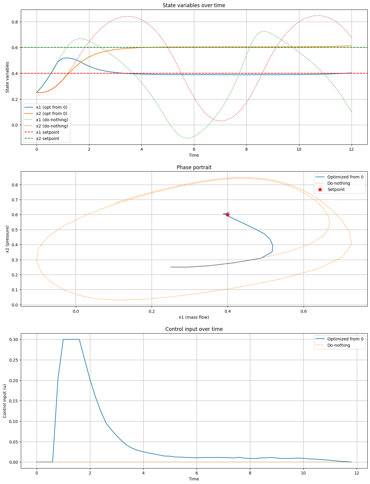
In the experiment below, we choose the setpoint \(\mathbf{x}^* = [0.40, 0.60]^T\) as it corresponds to an unstable equilibrium point. If we were to run the system without applying any control, we would see that the system starts to oscillate.
Show code cell source
import numpy as np
from scipy.optimize import minimize
import matplotlib.pyplot as plt

# System parameters
gamma, B, H, psi_c0, W = 0.5, 1, 0.18, 0.3, 0.25
alpha, beta, kappa, R = 1, 0, 0.08, 0
T, N = 12, 60
dt = T / N
x1_star, x2_star = 0.40, 0.60

def psi_e(x1):
    return psi_c0 + H * (1 + 1.5 * ((x1 / W) - 1) - 0.5 * ((x1 / W) - 1)**3)

def phi(x2):
    return gamma * np.sign(x2) * np.sqrt(np.abs(x2))

def system_dynamics(x, u):
    x1, x2 = x
    dx1dt = B * (psi_e(x1) - x2 - u)
    dx2dt = (1 / B) * (x1 - phi(x2))
    return np.array([dx1dt, dx2dt])

def euler_step(x, u, dt):
    return x + dt * system_dynamics(x, u)

def instantenous_cost(x, u):
    return (alpha * np.sum((x - np.array([x1_star, x2_star]))**2) + kappa * u**2)

def terminal_cost(x):
    return beta * np.sum((x - np.array([x1_star, x2_star]))**2)

def objective_and_constraints(z):
    u, v = z[:-1], z[-1]
    x = np.zeros((N+1, 2))
    x[0] = x0
    obj = 0
    cons = []
    for i in range(N):
        x[i+1] = euler_step(x[i], u[i], dt)
        obj += dt * instantenous_cost(x[i], u[i])
        cons.append(0.4 - x[i+1, 1] - v)
    obj += terminal_cost(x[-1]) + R * v**2
    return obj, np.array(cons)

def solve_trajectory_optimization(x0, u_init):
    z0 = np.zeros(N + 1)
    z0[:-1] = u_init
    bounds = [(0, 0.3)] * N + [(0, None)]
    result = minimize(
        lambda z: objective_and_constraints(z)[0],
        z0,
        method='SLSQP',
        bounds=bounds,
        constraints={'type': 'ineq', 'fun': lambda z: -objective_and_constraints(z)[1]},
        options={'disp': True, 'maxiter': 1000, 'ftol': 1e-6}
    )
    return result.x, result

def simulate_trajectory(x0, u):
    x = np.zeros((N+1, 2))
    x[0] = x0
    for i in range(N):
        x[i+1] = euler_step(x[i], u[i], dt)
    return x

# Run optimizations and simulations
x0 = np.array([0.25, 0.25])
t = np.linspace(0, T, N+1)

# Optimized control starting from zero
z_single_shooting, _ = solve_trajectory_optimization(x0, np.zeros(N))
u_opt_shoot, v_opt_shoot = z_single_shooting[:-1], z_single_shooting[-1]
x_opt_shoot = simulate_trajectory(x0, u_opt_shoot)

# Do-nothing control (u = 0)
u_nothing = np.zeros(N)
x_nothing = simulate_trajectory(x0, u_nothing)

# Plotting
plt.figure(figsize=(15, 20))

# State variables over time
plt.subplot(3, 1, 1)
plt.plot(t, x_opt_shoot[:, 0], label='x1 (opt from 0)')
plt.plot(t, x_opt_shoot[:, 1], label='x2 (opt from 0)')
plt.plot(t, x_nothing[:, 0], ':', label='x1 (do-nothing)')
plt.plot(t, x_nothing[:, 1], ':', label='x2 (do-nothing)')
plt.axhline(y=x1_star, color='r', linestyle='--', label='x1 setpoint')
plt.axhline(y=x2_star, color='g', linestyle='--', label='x2 setpoint')
plt.xlabel('Time')
plt.ylabel('State variables')
plt.title('State variables over time')
plt.legend()
plt.grid(True)

# Phase portrait
plt.subplot(3, 1, 2)
plt.plot(x_opt_shoot[:, 0], x_opt_shoot[:, 1], label='Optimized from 0')
plt.plot(x_nothing[:, 0], x_nothing[:, 1], ':', label='Do-nothing')
plt.plot(x1_star, x2_star, 'r*', markersize=10, label='Setpoint')
plt.xlabel('x1 (mass flow)')
plt.ylabel('x2 (pressure)')
plt.title('Phase portrait')
plt.legend()
plt.grid(True)

# Control inputs
plt.subplot(3, 1, 3)
plt.plot(t[:-1], u_opt_shoot, label='Optimized from 0')
plt.plot(t[:-1], u_nothing, ':', label='Do-nothing')
plt.xlabel('Time')
plt.ylabel('Control input (u)')
plt.title('Control input over time')
plt.legend()
plt.grid(True)
Optimization terminated successfully    (Exit mode 0)
            Current function value: 0.17449650818410942
            Iterations: 37
            Function evaluations: 2306
            Gradient evaluations: 37
Solution by Trapezoidal Collocation#
Another way to pose the problem is by imposing a terminal state constraint on the system rather than through a penalty in the integral term. In the following experiment, we use a problem formulation of the form:
We then find a control function \(u(t)\) and state trajectory \(x(t)\) using the trapezoidal collocation method.
Show code cell source
import numpy as np
from scipy.optimize import minimize
from scipy.integrate import solve_ivp
from scipy.interpolate import interp1d
import matplotlib.pyplot as plt

# System parameters
gamma, B, H, psi_c0, W = 0.5, 1, 0.18, 0.3, 0.25
kappa = 0.08
T, N = 12, 20  # Number of collocation points
t = np.linspace(0, T, N)
dt = T / (N - 1)
x1_star, x2_star = 0.40, 0.60

def psi_e(x1):
    return psi_c0 + H * (1 + 1.5 * ((x1 / W) - 1) - 0.5 * ((x1 / W) - 1)**3)

def phi(x2):
    return gamma * np.sign(x2) * np.sqrt(np.abs(x2))

def system_dynamics(t, x, u_func):
    x1, x2 = x
    u = u_func(t)
    dx1dt = B * (psi_e(x1) - x2 - u)
    dx2dt = (1 / B) * (x1 - phi(x2))
    return [dx1dt, dx2dt]

def objective(z):
    x = z[:2*N].reshape((N, 2))
    u = z[2*N:]

    # Trapezoidal rule for the cost function
    cost = 0
    for i in range(N-1):
        cost += 0.5 * dt * (kappa * u[i]**2 + kappa * u[i+1]**2)

    return cost

def constraints(z):
    x = z[:2*N].reshape((N, 2))
    u = z[2*N:]

    cons = []

    # Dynamics constraints (trapezoidal rule)
    for i in range(N-1):
        f_i = system_dynamics(t[i], x[i], lambda t: u[i])
        f_ip1 = system_dynamics(t[i+1], x[i+1], lambda t: u[i+1])
        cons.extend(x[i+1] - x[i] - 0.5 * dt * (np.array(f_i) + np.array(f_ip1)))

    # Terminal constraint
    cons.extend([x[-1, 0] - x1_star, x[-1, 1] - x2_star])

    # Initial condition constraint
    cons.extend([x[0, 0] - x0[0], x[0, 1] - x0[1]])

    return np.array(cons)

def solve_trajectory_optimization(x0):
    # Initial guess
    x_init = np.linspace(x0, [x1_star, x2_star], N)
    u_init = np.zeros(N)
    z0 = np.concatenate([x_init.flatten(), u_init])

    # Bounds
    bounds = [(None, None)] * (2*N)  # State variables
    bounds += [(0, 0.3)] * N  # Control inputs

    # Constraints
    cons = {'type': 'eq', 'fun': constraints}

    result = minimize(
        objective,
        z0,
        method='SLSQP',
        bounds=bounds,
        constraints=cons,
        options={'disp': True, 'maxiter': 1000, 'ftol': 1e-6}
    )
    return result.x, result

# Run optimization
x0 = np.array([0.5, 0.5])
z_opt, result = solve_trajectory_optimization(x0)
x_opt_coll = z_opt[:2*N].reshape((N, 2))
u_opt_coll = z_opt[2*N:]

print(f"Optimization successful: {result.success}")
print(f"Final objective value: {result.fun}")
print(f"Final state: x1 = {x_opt_coll[-1, 0]:.4f}, x2 = {x_opt_coll[-1, 1]:.4f}")
print(f"Target state: x1 = {x1_star:.4f}, x2 = {x2_star:.4f}")

# Create interpolated control function
u_func = interp1d(t, u_opt_coll, kind='linear', bounds_error=False, fill_value=(u_opt_coll[0], u_opt_coll[-1]))

# Solve IVP with the optimized control
sol = solve_ivp(lambda t, x: system_dynamics(t, x, u_func), [0, T], x0, dense_output=True)

# Generate solution points
t_dense = np.linspace(0, T, 200)
x_ivp = sol.sol(t_dense).T

# Plotting
plt.figure(figsize=(15, 20))

# State variables over time
plt.subplot(3, 1, 1)
plt.plot(t, x_opt_coll[:, 0], 'bo-', label='x1 (collocation)')
plt.plot(t, x_opt_coll[:, 1], 'ro-', label='x2 (collocation)')
plt.plot(t_dense, x_ivp[:, 0], 'b--', label='x1 (integrated)')
plt.plot(t_dense, x_ivp[:, 1], 'r--', label='x2 (integrated)')
plt.axhline(y=x1_star, color='b', linestyle=':', label='x1 setpoint')
plt.axhline(y=x2_star, color='r', linestyle=':', label='x2 setpoint')
plt.xlabel('Time')
plt.ylabel('State variables')
plt.title('State variables over time')
plt.legend()
plt.grid(True)

# Phase portrait
plt.subplot(3, 1, 2)
plt.plot(x_opt_coll[:, 0], x_opt_coll[:, 1], 'go-', label='Collocation')
plt.plot(x_ivp[:, 0], x_ivp[:, 1], 'm--', label='Integrated')
plt.plot(x1_star, x2_star, 'r*', markersize=10, label='Setpoint')
plt.xlabel('x1 (mass flow)')
plt.ylabel('x2 (pressure)')
plt.title('Phase portrait')
plt.legend()
plt.grid(True)

# Control inputs
plt.subplot(3, 1, 3)
plt.step(t, u_opt_coll, 'g-', where='post', label='Collocation')
plt.plot(t_dense, u_func(t_dense), 'm--', label='Interpolated')
plt.xlabel('Time')
plt.ylabel('Control input (u)')
plt.title('Control input over time')
plt.legend()
plt.grid(True)

plt.tight_layout()
plt.show()
Optimization terminated successfully    (Exit mode 0)
            Current function value: 0.0023543222096489565
            Iterations: 13
            Function evaluations: 794
            Gradient evaluations: 13
Optimization successful: True
Final objective value: 0.0023543222096489565
Final state: x1 = 0.4000, x2 = 0.6000
Target state: x1 = 0.4000, x2 = 0.6000
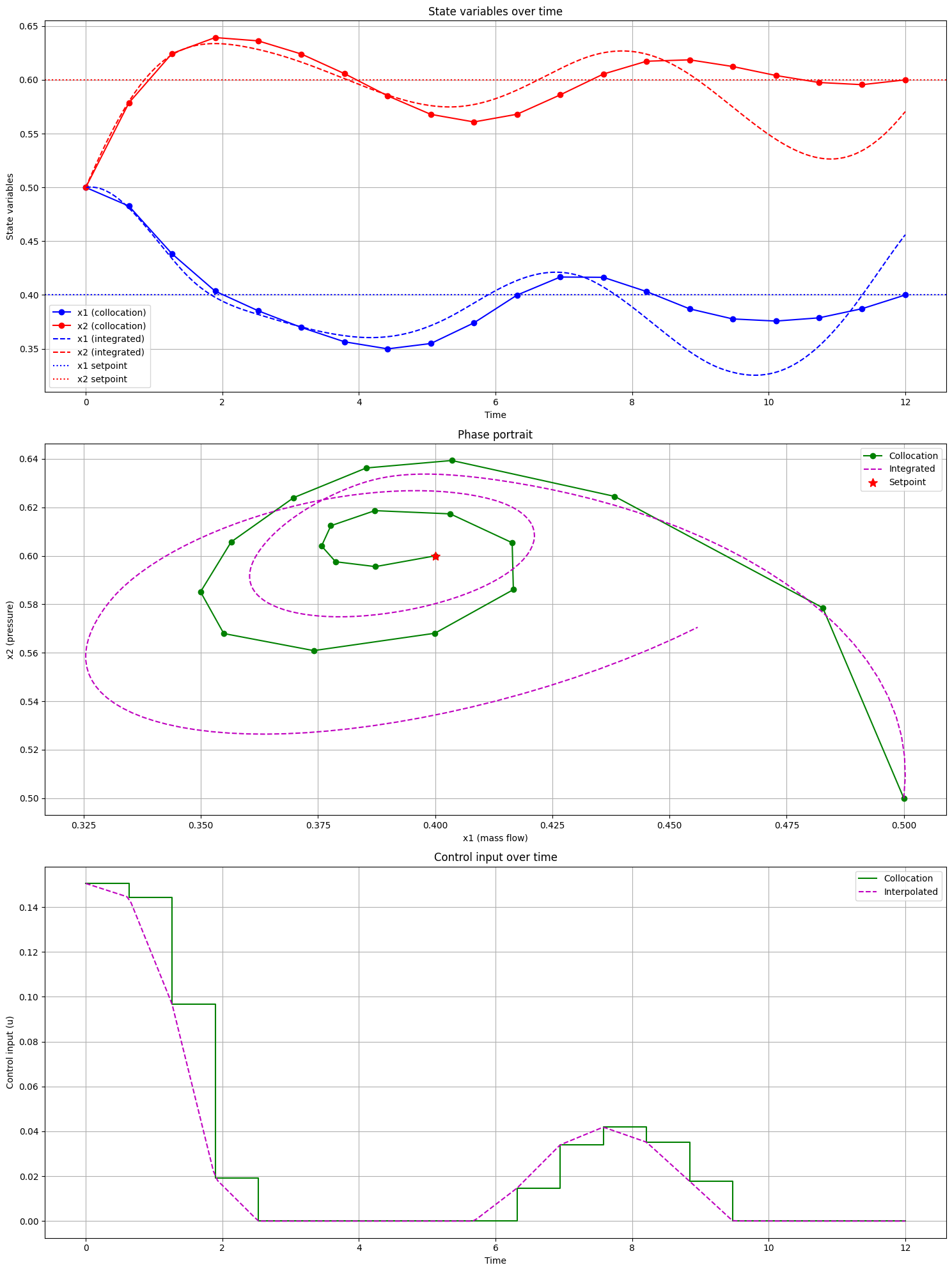
You can try to vary the number of collocation points in the code and observe how the state trajectory progressively matches the ground truth (the line denoted “integrated solution”). Note that this version of the code also lacks bound constraints on the variable \(x_2\) to ensure a minimum pressure, as we did earlier. Consider this a good exercise to try on your own.
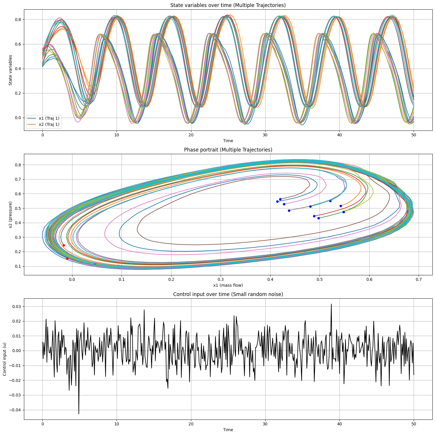
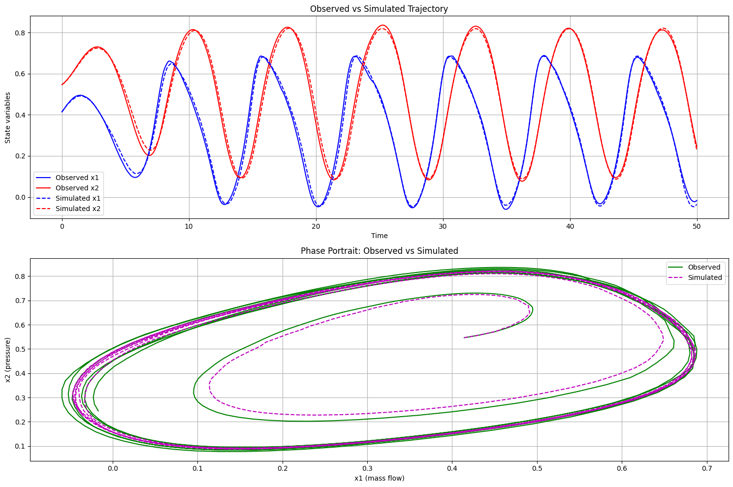
System Identification as Trajectory Optimization (Compressor Surge)#
We now turn the compressor surge model into a simple system identification task: estimate unknown parameters (here, the scalar \(B\)) from measured trajectories. This can be viewed as a trajectory optimization problem: choose parameters (and optionally states) to minimize reconstruction error while enforcing the dynamics.
Given time-aligned data \(\{(\mathbf{u}_k,\mathbf{y}_k)\}_{k=0}^{N}\), model states \(\mathbf{x}_k\in\mathbb{R}^d\), outputs \(\mathbf{y}_k\approx \mathbf{h}(\mathbf{x}_k;\boldsymbol{\theta})\), step \(\Delta t\), and dynamics \(\mathbf{f}(\mathbf{x},\mathbf{u};\boldsymbol{\theta})\), the simultaneous (full-discretization) viewpoint is
while the single-shooting (recursive elimination) variant eliminates the states by simulating forward from \(\mathbf{x}_0\):
where \(\boldsymbol{\phi}_k\) denotes the state reached at step \(k\) by an RK4 rollout under parameter \(\boldsymbol{\theta}\). In our demo the data grid and rollout grid coincide, so \(\boldsymbol{\phi}_k = \mathbf{x}_k\) and no interpolation is required. We will identify \(B\) by fitting the model to data generated from the ground-truth \(B=1\) system under randomized initial conditions and small input perturbations.
Show code cell source
import numpy as np
from scipy.integrate import solve_ivp
import matplotlib.pyplot as plt

# System parameters
gamma, B, H, psi_c0, W = 0.5, 1, 0.18, 0.3, 0.25

# Simulation parameters
T = 50  # Total simulation time
dt = 0.1  # Time step
t = np.arange(0, T + dt, dt)
N = len(t)

# Number of trajectories
num_trajectories = 10

def psi_e(x1):
    return psi_c0 + H * (1 + 1.5 * ((x1 / W) - 1) - 0.5 * ((x1 / W) - 1)**3)

def phi(x2):
    return gamma * np.sign(x2) * np.sqrt(np.abs(x2))

def system_dynamics(t, x, u):
    x1, x2 = x
    dx1dt = B * (psi_e(x1) - x2 - u)
    dx2dt = (1 / B) * (x1 - phi(x2))
    return [dx1dt, dx2dt]

# "Do nothing" controller with small random noise
def u_func(t):
    return np.random.normal(0, 0.01)  # Mean 0, standard deviation 0.01

# Function to simulate a single trajectory
def simulate_trajectory(x0):
    sol = solve_ivp(lambda t, x: system_dynamics(t, x, u_func(t)), [0, T], x0, t_eval=t, method='RK45')
    return sol.y[0], sol.y[1]

# Generate multiple trajectories
trajectories = []
initial_conditions = []

for i in range(num_trajectories):
    # Randomize initial conditions around [0.5, 0.5]
    x0 = np.array([0.5, 0.5]) + np.random.normal(0, 0.05, 2)
    initial_conditions.append(x0)
    x1, x2 = simulate_trajectory(x0)
    trajectories.append((x1, x2))

# Calculate control inputs (small random noise)
u = np.array([u_func(ti) for ti in t])

# Plotting
plt.figure(figsize=(15, 15))

# State variables over time
plt.subplot(3, 1, 1)
for i, (x1, x2) in enumerate(trajectories):
    plt.plot(t, x1, label=f'x1 (Traj {i+1})' if i == 0 else "_nolegend_")
    plt.plot(t, x2, label=f'x2 (Traj {i+1})' if i == 0 else "_nolegend_")
plt.xlabel('Time')
plt.ylabel('State variables')
plt.title('State variables over time (Multiple Trajectories)')
plt.legend()
plt.grid(True)

# Phase portrait
plt.subplot(3, 1, 2)
for x1, x2 in trajectories:
    plt.plot(x1, x2)
    plt.plot(x1[0], x2[0], 'bo', markersize=5)
    plt.plot(x1[-1], x2[-1], 'ro', markersize=5)
plt.xlabel('x1 (mass flow)')
plt.ylabel('x2 (pressure)')
plt.title('Phase portrait (Multiple Trajectories)')
plt.grid(True)

# Control input (small random noise)
plt.subplot(3, 1, 3)
plt.plot(t, u, 'k-')
plt.xlabel('Time')
plt.ylabel('Control input (u)')
plt.title('Control input over time (Small random noise)')
plt.grid(True)

plt.tight_layout()
plt.show()

# Save the data
np.savez('_static/compressor_surge_data_multi.npz', t=t, trajectories=trajectories, u=u, initial_conditions=initial_conditions)

print("Data collection complete. Results saved to 'compressor_surge_data_multi.npz'")
print(f"Data shape: {num_trajectories} trajectories, each with {N} time steps")
print(f"Time range: 0 to {T} seconds")
print("Initial conditions:")
for i, x0 in enumerate(initial_conditions):
    print(f"  Trajectory {i+1}: x1 = {x0[0]:.4f}, x2 = {x0[1]:.4f}")
Data collection complete. Results saved to 'compressor_surge_data_multi.npz'
Data shape: 10 trajectories, each with 501 time steps
Time range: 0 to 50 seconds
Initial conditions:
  Trajectory 1: x1 = 0.4142, x2 = 0.5466
  Trajectory 2: x1 = 0.5425, x2 = 0.5155
  Trajectory 3: x1 = 0.4976, x2 = 0.4306
  Trajectory 4: x1 = 0.4886, x2 = 0.4448
  Trajectory 5: x1 = 0.5209, x2 = 0.5508
  Trajectory 6: x1 = 0.4202, x2 = 0.5627
  Trajectory 7: x1 = 0.4281, x2 = 0.5283
  Trajectory 8: x1 = 0.4378, x2 = 0.4846
  Trajectory 9: x1 = 0.5485, x2 = 0.4747
  Trajectory 10: x1 = 0.4811, x2 = 0.5120
Show code cell source
import numpy as np
from scipy.optimize import minimize
import matplotlib.pyplot as plt

# Load the data
data = np.load('_static/compressor_surge_data_multi.npz', allow_pickle=True)
t = data['t']
trajectories = data['trajectories']
u = data['u']
initial_conditions = data['initial_conditions']

# Known system parameters
gamma, H, psi_c0, W = 0.5, 0.18, 0.3, 0.25
# B is the parameter we want to identify
B_true = 1.0  # True value, used for comparison

def psi_e(x1):
    return psi_c0 + H * (1 + 1.5 * ((x1 / W) - 1) - 0.5 * ((x1 / W) - 1)**3)

def phi(x2):
    return gamma * np.sign(x2) * np.sqrt(np.abs(x2))

def system_dynamics(t, x, u, B):
    x1, x2 = x
    dx1dt = B * (psi_e(x1) - x2 - u)
    dx2dt = (1 / B) * (x1 - phi(x2))
    return np.array([dx1dt, dx2dt])

def rk4_step(f, t, x, u, dt, B):
    k1 = f(t, x, u, B)
    k2 = f(t + 0.5*dt, x + 0.5*dt*k1, u, B)
    k3 = f(t + 0.5*dt, x + 0.5*dt*k2, u, B)
    k4 = f(t + dt, x + dt*k3, u, B)
    return x + (dt/6) * (k1 + 2*k2 + 2*k3 + k4)

def simulate_trajectory(x0, B):
    x = np.zeros((len(t), 2))
    x[0] = x0
    for i in range(1, len(t)):
        x[i] = rk4_step(system_dynamics, t[i-1], x[i-1], u[i-1], t[i] - t[i-1], B)
    return x

def objective(B):
    error = 0
    for i, (x1_obs, x2_obs) in enumerate(trajectories):
        x_sim = simulate_trajectory(initial_conditions[i], B[0])
        error += np.sum((x_sim[:, 0] - x1_obs)**2 + (x_sim[:, 1] - x2_obs)**2)
    return error

# Perform optimization
result = minimize(objective, x0=[1.5], method='Nelder-Mead', options={'disp': True})

B_identified = result.x[0]

print(f"True B: {B_true}")
print(f"Identified B: {B_identified}")
print(f"Relative error: {abs(B_identified - B_true) / B_true * 100:.2f}%")

# Plot results
plt.figure(figsize=(15, 10))

# Plot one trajectory for comparison
traj_index = 0
x1_obs, x2_obs = trajectories[traj_index]
x_sim = simulate_trajectory(initial_conditions[traj_index], B_identified)

plt.subplot(2, 1, 1)
plt.plot(t, x1_obs, 'b-', label='Observed x1')
plt.plot(t, x2_obs, 'r-', label='Observed x2')
plt.plot(t, x_sim[:, 0], 'b--', label='Simulated x1')
plt.plot(t, x_sim[:, 1], 'r--', label='Simulated x2')
plt.xlabel('Time')
plt.ylabel('State variables')
plt.title('Observed vs Simulated Trajectory')
plt.legend()
plt.grid(True)

plt.subplot(2, 1, 2)
plt.plot(x1_obs, x2_obs, 'g-', label='Observed')
plt.plot(x_sim[:, 0], x_sim[:, 1], 'm--', label='Simulated')
plt.xlabel('x1 (mass flow)')
plt.ylabel('x2 (pressure)')
plt.title('Phase Portrait: Observed vs Simulated')
plt.legend()
plt.grid(True)

plt.tight_layout()
plt.show()
Optimization terminated successfully.
         Current function value: 6.037293
         Iterations: 15
         Function evaluations: 30
True B: 1.0
Identified B: 1.0107421874999987
Relative error: 1.07%
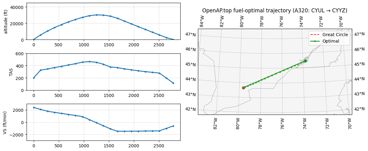
Flight Trajectory Optimization#
We consider a concrete task: computing a fuel-optimal trajectory between Montréal–Trudeau (CYUL) and Toronto Pearson (CYYZ), taking into account both aircraft dynamics and wind conditions along the route. For this demo, we leverage the excellent library OpenAP.top which provides direct transcription methods and airplane dynamics models [41]. Furthermore, it allows us to import a a wind field comes from ERA5 [46], a global atmospheric dataset. It combines historical observations from satellites, aircraft, and surface stations with a weather model to reconstruct the state of the atmosphere across space and time. In climate science, this is called a reanalysis.
ERA5 data is stored in GRIB files, a compact format widely used in meteorology. Each file contains a gridded field: values of wind and other variables arranged on a regular 4D lattice over longitude, latitude, altitude, and time. Since the aircraft rarely sits exactly on a grid point, we interpolate the wind components it sees as it moves.
The aircraft is modeled as a point mass with state
where \((x, y)\) is horizontal position, \(h\) is altitude, and \(m\) is remaining mass. Controls are Mach number \(M(t)\), vertical speed \(v_s(t)\), and heading angle \(\psi(t)\). The equations of motion combine airspeed and wind:
where \(\gamma = \arcsin(v_s / v)\) is the flight path angle and \(\mathrm{FF}\) is the fuel flow rate based on current conditions. The wind terms \(u_w\) and \(v_w\) are taken from ERA5 and interpolated in space and time.
The optimization minimizes fuel burn over the CYUL–CYYZ leg. But the same setup could be used to minimize arrival time, or some weighted combination of time, cost, and emissions.
We use OpenAP.top, which solves the problem using direct collocation at Legendre–Gauss–Lobatto (LGL) points. Each trajectory segment is mapped to the unit interval, the state is interpolated by Lagrange polynomials at nonuniform LGL nodes, and the dynamics are enforced at those points. Integration is done with matching quadrature weights.
This setup lets us optimize trajectories under realistic conditions by feeding in the appropriate ERA5 GRIB file (e.g., era5_mtl_20230601_12.grib). The result accounts for wind patterns (eg. headwinds, tailwinds, shear) along the corridor between Montréal and Toronto.
Show code cell source
# OpenAP.top demo with optional wind overlay – docs: https://github.com/junzis/openap-top
from openap import top
import matplotlib.pyplot as plt
import os

# Montreal region route (Canada): CYUL (Montréal–Trudeau) → CYYZ (Toronto)
opt = top.CompleteFlight("A320", "CYUL", "CYYZ", m0=0.85)

# Optional: point to a local ERA5/GRIB file to enable wind (set env var OPENAP_WIND_GRIB)
# If not set, look for a default small file produced by `_static/openap_fetch_era5.py`.
fgrib = os.environ.get("OPENAP_WIND_GRIB", "_static/era5_mtl_20230601_12.grib")
windfield = None
if fgrib and os.path.exists(fgrib):
    try:
        windfield = top.tools.read_grids(fgrib)
        opt.enable_wind(windfield)
    except Exception:
        windfield = None  # fall back silently if GRIB reading deps are missing

# Solve for a fuel-optimal trajectory (CasADi direct collocation under the hood)
flight = opt.trajectory(objective="fuel")

# Visualize; overlay wind barbs if windfield available
if windfield is not None:
    ax = top.vis.trajectory(flight, windfield=windfield, barb_steps=15)
else:
    ax = top.vis.trajectory(flight)

title = "OpenAP.top fuel-optimal trajectory (A320: CYUL → CYYZ)"
if hasattr(ax, "set_title"):
    ax.set_title(title)
else:
    plt.title(title)
Hydro Cascade Scheduling with Physical Routing and Multiple Shooting#
Earlier in the book, we introduced a simplified view of hydro reservoir control, where the water level evolves in discrete time by accounting for inflow and outflow, with precipitation treated as a noisy input. While useful for learning and control design, this model abstracts away much of the physical behavior of actual rivers and dams.
In this chapter, we move toward a more realistic setup inspired by [39]. We consider a series of dams arranged in a cascade, where the actions taken upstream influence downstream levels with a delay. The amount of power produced depends not only on how much water flows through the turbines, but also on the head (the vertical distance between the reservoir surface and the turbine outlet). The larger the head, the more potential energy is available for conversion into electricity, and the higher the power output.
To capture these effects, we follow a modeling approach inspired by the Saint-Venant equations, which describe how water levels and flows evolve in open channels. Instead of solving the full PDEs, we use a reduced model that approximates each dammed section of river (called a reach) as a lumped system governed by an ordinary differential equation. The main variable of interest is the water level \(h_r(t)\), which changes over time depending on how much water enters, how much is discharged through the turbines \(q_r(t)\), and how much is spilled \(s_r(t)\). The mass balance for reach \(r\) is written as:
where \(A_r\) is the surface area of the reservoir, assumed constant. The inflow \(z_r(t)\) to a reach either comes from nature (for the first dam), or from the upstream turbine and spill discharge, delayed by a travel time \(\tau_{r-1}\):
Power generation at each reach depends on how much water is discharged and the available head:
where \(\rho\) is water density, \(g\) is gravitational acceleration, \(\eta\) is turbine efficiency, and \(H_r(h_r(t))\) denotes the head as a function of the water level. In some models, the head is approximated as the difference between the current level and a fixed tailwater height (the water level downstream of the dam, after it has passed through the turbine).
The operator’s goal is to meet a target generation profile \(P^\text{ref}(t)\), such as one dictated by a market dispatch or load-following constraint. This leads to an objective that minimizes the deviation from the target over the full horizon:
In practice, this is combined with operational constraints: turbine capacity \(0 \le q_r(t) \le \bar{q}_r\), spillway limits \(0 \le s_r(t) \le \bar{s}_r\), and safe level bounds \(h_r^{\min} \le h_r(t) \le h_r^{\max}\). Depending on the use case, one may also penalize spill to encourage water conservation, or penalize fast changes in levels for ecological reasons.
What makes this problem particularly interesting is the coupling across space and time. An upstream reach cannot simply act in isolation: if the operator wants reach \(r\) to produce power at a specific time, the water must be released by reach \(r-1\) sufficiently in advance. This coordination is further complicated by delays, nonlinearities in head-dependent power, and limited storage capacity.
We solve the problem using multiple shooting. Each reach is divided into local simulation segments over short time windows. Within each segment, the dynamics are integrated forward using the ODEs, and continuity constraints are added to ensure that the water levels match across segment boundaries. At the same time, the inflows passed from upstream reaches must arrive at the right time and be consistent with previous decisions. In discrete time, this gives rise to a set of state-update equations:
with delays handled by shifting \(z_r^k\) according to the appropriate travel time. These constraints are enforced as part of a nonlinear program, alongside the power tracking objective and control bounds.
Compared to the earlier inflow-outflow model, this richer setup introduces more structure, but also more opportunity. The cascade now behaves like a coordinated team: upstream reservoirs can store water in anticipation of future needs, while downstream dams adjust their output to match arrivals and avoid overflows. The optimization reveals not just a schedule, but a strategy for how the entire system should act together to meet demand.
Show code cell source
# Instrumented MSD hydro demo with heterogeneity + diagnostics
# - Breaks symmetry to avoid trivial identical plots
# - Adds rich diagnostics to explain flat levels and equalities
#
# This cell runs end-to-end and shows plots + tables.

import numpy as np
import pandas as pd
import matplotlib.pyplot as plt
from dataclasses import dataclass
from typing import Tuple
from scipy.optimize import minimize
from math import sqrt
import warnings

# ---------- Model ----------

g = 9.81  # m/s^2

@dataclass
class ReachParams:
    L: float
    W: float
    k_b: float
    S_b: float
    k_t: float
    @property
    def A_surf(self) -> float:
        return self.L * self.W

def smooth_relu(x, eps=1e-9):
    return 0.5*(x + np.sqrt(x*x + eps))

def q_bypass(H, rp: ReachParams):
    H_eff = smooth_relu(H)
    return rp.k_b * rp.S_b * np.sqrt(2*g*H_eff)

def muskingum_coeffs(K: float, X: float, dt: float) -> Tuple[float, float, float]:
    D  = 2.0*K*(1.0 - X) + dt
    C0 = (dt - 2.0*K*X) / D
    C1 = (dt + 2.0*K*X) / D
    C2 = (2.0*K*(1.0 - X) - dt) / D
    return C0, C1, C2

def integrate_interval(H0, u, z, dt, nsub, rp: ReachParams):
    """Forward Euler. Returns Hend, avg_qout."""
    h = dt/nsub
    H = H0
    qsum = 0.0
    for _ in range(nsub):
        qb = q_bypass(H, rp)
        qout = u + qb
        dHdt = (z - qout) / rp.A_surf
        H += h*dHdt
        qsum += qout
    return H, qsum/nsub

def shapes(M,N): return (M*(N+1), M*N, M*N)

def unpack(x, M, N):
    nH, nu, nz = shapes(M,N)
    H = x[:nH].reshape(M,N+1)
    u = x[nH:nH+nu].reshape(M,N)
    z = x[nH+nu:nH+nu+nz].reshape(M,N)
    return H,u,z

def pack(H,u,z): return np.concatenate([H.ravel(), u.ravel(), z.ravel()])

# ---------- Problem builder ----------

def make_params_hetero(M):
    """Heterogeneous reaches to break symmetry."""
    # Widths, spillway areas, and power coeffs vary by reach
    W_list = np.linspace(80, 140, M)         # m
    L_list = np.full(M, 4000.0)              # m
    S_b_list = np.linspace(14.0, 20.0, M)    # m^2
    k_t_list = np.linspace(7.5, 8.5, M)      # power coeff
    k_b_list = np.linspace(0.55, 0.65, M)    # spill coeff
    return [ReachParams(L=float(L_list[i]), W=float(W_list[i]),
                        k_b=float(k_b_list[i]), S_b=float(S_b_list[i]),
                        k_t=float(k_t_list[i])) for i in range(M)]

def build_demo(M=3, N=12, dt=900.0, seed=0, hetero=True):
    rng = np.random.default_rng(seed)
    params = make_params_hetero(M) if hetero else [ReachParams(4000.0, 100.0, 0.6, 18.26, 8.0) for _ in range(M)]

    # initial levels (heterogeneous)
    H0 = np.array([17.0, 16.7, 17.3][:M])

    H_ref = np.array([17.0, 16.9, 17.1][:M]) if hetero else np.full(M, 17.0)
    H_bounds = (16.0, 18.5)
    u_bounds = (40.0, 160.0)

    Qin_base = 300.0
    Qin_ext = Qin_base + 30.0*np.sin(2*np.pi*np.arange(N)/N)  # stronger swing

    Pref_raw = 60.0 + 15.0*np.sin(2*np.pi*(np.arange(N)-2)/N)

    # default Muskingum parameters per link (M-1 links)
    if M > 1:
        K_list = list(np.linspace(1800.0, 2700.0, M-1))
        X_list = [0.2]*(M-1)
    else:
        K_list = []
        X_list = []

    return dict(params=params, H0=H0, H_ref=H_ref, H_bounds=H_bounds,
                u_bounds=u_bounds, Qin_ext=Qin_ext, Pref_raw=Pref_raw,
                dt=dt, N=N, M=M, nsub=10,
                muskingum=dict(K=K_list, X=X_list))

# ---------- Objective / constraints / helpers ----------

def compute_total_power(H,u,params):
    M,N = u.shape
    Pn = np.zeros(N)
    for n in range(N):
        for i in range(M):
            Pn[n] += params[i].k_t * u[i,n] * H[i,n]
    return Pn

def decompose_objective(x, data, Pref, wP, wH, wDu):
    H,u,z = unpack(x, data["M"], data["N"])
    params, H_ref = data["params"], data["H_ref"]
    track = np.sum((compute_total_power(H,u,params)-Pref)**2)
    lvl   = np.sum((H[:,:-1]-H_ref[:,None])**2)
    du    = np.sum((u[:,1:]-u[:,:-1])**2)
    return dict(track=wP*track, lvl=wH*lvl, du=wDu*du, raw=dict(track=track,lvl=lvl,du=du))

def make_objective(data, Pref, wP=8.0, wH=0.02, wDu=1e-4):
    params, H_ref, N, M = data["params"], data["H_ref"], data["N"], data["M"]
    def obj(x):
        H,u,z = unpack(x,M,N)
        return (
            wP*np.sum((compute_total_power(H,u,params)-Pref)**2)
            + wH*np.sum((H[:,:-1]-H_ref[:,None])**2)
            + wDu*np.sum((u[:,1:]-u[:,:-1])**2)
        )
    return obj, dict(wP=wP,wH=wH,wDu=wDu)

def make_constraints(data):
    params, H0, Qin_ext, dt, N, M, nsub = (
        data["params"], data["H0"], data["Qin_ext"], data["dt"], data["N"], data["M"], data["nsub"]
    )
    cons = []
    def init_fun(x):
        H,u,z = unpack(x,M,N); return H[:,0]-H0
    cons.append({'type':'eq','fun':init_fun})
    def dyn_fun(x):
        H,u,z = unpack(x,M,N)
        res=[]
        for i in range(M):
            for n in range(N):
                Hend, _ = integrate_interval(H[i,n], u[i,n], z[i,n], dt, nsub, params[i])
                res.append(H[i,n+1]-Hend)
        return np.array(res)
    cons.append({'type':'eq','fun':dyn_fun})
    def coup_fun(x):
        H,u,z = unpack(x,M,N)
        res=[]
        # First reach is exogenous inflow per interval
        for n in range(N):
            res.append(z[0,n]-Qin_ext[n])
        # Downstream links: Muskingum routing
        K_list = data.get("muskingum", {}).get("K", [])
        X_list = data.get("muskingum", {}).get("X", [])
        for i in range(1,M):
            # Seed condition for z[i,0]
            _, I0 = integrate_interval(H[i-1,0], u[i-1,0], z[i-1,0], dt, nsub, params[i-1])
            res.append(z[i,0] - I0)
            # Coefficients
            Ki = K_list[i-1] if i-1 < len(K_list) else 1800.0
            Xi = X_list[i-1] if i-1 < len(X_list) else 0.2
            C0, C1, C2 = muskingum_coeffs(Ki, Xi, dt)
            # Recursion over intervals
            for n in range(N-1):
                # upstream interval-average outflows for n and n+1
                _, I_n   = integrate_interval(H[i-1,n],   u[i-1,n],   z[i-1,n],   dt, nsub, params[i-1])
                _, I_np1 = integrate_interval(H[i-1,n+1], u[i-1,n+1], z[i-1,n+1], dt, nsub, params[i-1])
                res.append(z[i,n+1] - (C0*I_np1 + C1*I_n + C2*z[i,n]))
        return np.array(res)
    cons.append({'type':'eq','fun':coup_fun})
    return cons

def make_bounds(data):
    Hmin,Hmax = data["H_bounds"]
    umin,umax = data["u_bounds"]
    M,N = data["M"], data["N"]
    nH,nu,nz = shapes(M,N)
    lb = np.empty(nH+nu+nz); ub = np.empty_like(lb)
    lb[:nH]=Hmin; ub[:nH]=Hmax
    lb[nH:nH+nu]=umin; ub[nH:nH+nu]=umax
    lb[nH+nu:]=0.0; ub[nH+nu:]=2000.0
    return list(zip(lb,ub))

def residuals(x, data):
    params, H0, Qin_ext, dt, N, M, nsub = (
        data["params"], data["H0"], data["Qin_ext"], data["dt"], data["N"], data["M"], data["nsub"]
    )
    H,u,z = unpack(x, M, N)
    dyn = np.zeros((M,N)); coup = np.zeros((M,N))
    for i in range(M):
        for n in range(N):
            Hend, qavg = integrate_interval(H[i,n], u[i,n], z[i,n], dt, nsub, params[i])
            dyn[i,n] = H[i,n+1] - Hend
            if i == 0:
                coup[i,n] = z[i,n] - Qin_ext[n]
            else:
                # Muskingum residual, align on current index using n and n-1
                Ki = data.get("muskingum", {}).get("K", [1800.0]*(M-1))[i-1]
                Xi = data.get("muskingum", {}).get("X", [0.2]*(M-1))[i-1]
                C0, C1, C2 = muskingum_coeffs(Ki, Xi, dt)
                if n == 0:
                    coup[i,n] = 0.0
                else:
                    _, I_nm1 = integrate_interval(H[i-1,n-1], u[i-1,n-1], z[i-1,n-1], dt, nsub, params[i-1])
                    _, I_n   = integrate_interval(H[i-1,n],   u[i-1,n],   z[i-1,n],   dt, nsub, params[i-1])
                    coup[i,n] = z[i,n] - (C0*I_n + C1*I_nm1 + C2*z[i,n-1])
    return dyn, coup

# ---------- Feasible initial guess with hetero controls ----------

def feasible_initial_guess(data):
    """Feasible x0 with nontrivial u by setting u at mid + per-reach pattern, then integrating to define H,z."""
    M,N,dt,nsub = data["M"], data["N"], data["dt"], data["nsub"]
    params = data["params"]
    umin,umax = data["u_bounds"]
    Qin_ext = data["Qin_ext"]

    # pattern to break symmetry
    base = 0.5*(umin+umax)
    phase = np.linspace(0, np.pi/2, M)
    tgrid = np.arange(N)
    u_pattern = np.array([base + 25*np.sin(2*np.pi*(tgrid/N) + ph) for ph in phase])
    u_pattern = np.clip(u_pattern, umin, umax)

    H = np.zeros((M, N+1)); u = np.zeros((M, N)); z = np.zeros((M, N))
    H[:,0] = data["H0"]
    # Set controls from pattern first
    for i in range(M):
        u[i,:] = u_pattern[i,:]

    # First reach: exogenous inflow, integrate forward and record outflow averages
    qavg_up = np.zeros((M, N))
    for n in range(N):
        z[0,n] = Qin_ext[n]
        Hend, qavg = integrate_interval(H[0,n], u[0,n], z[0,n], dt, nsub, params[0])
        H[0,n+1] = Hend
        qavg_up[0,n] = qavg

    # Downstream reaches with Muskingum routing
    K_list = data.get("muskingum", {}).get("K", [1800.0]*(M-1))
    X_list = data.get("muskingum", {}).get("X", [0.2]*(M-1))
    for i in range(1,M):
        Ki = K_list[i-1] if i-1 < len(K_list) else 1800.0
        Xi = X_list[i-1] if i-1 < len(X_list) else 0.2
        C0, C1, C2 = muskingum_coeffs(Ki, Xi, dt)
        I = qavg_up[i-1,:]
        # seed
        z[i,0] = I[0]
        # propagate recursively over time
        for n in range(N-1):
            z[i,n+1] = C0*I[n+1] + C1*I[n] + C2*z[i,n]
        # integrate levels for reach i using routed inflow
        for n in range(N):
            Hend, qavg = integrate_interval(H[i,n], u[i,n], z[i,n], dt, nsub, params[i])
            H[i,n+1] = Hend
            qavg_up[i,n] = qavg
    return pack(H,u,z)

def scale_pref(Pref_raw, x0, data):
    H,u,z = unpack(x0, data["M"], data["N"])
    P0 = compute_total_power(H,u,data["params"])
    s = max(np.mean(P0),1e-6)/max(np.mean(Pref_raw),1e-6)
    return Pref_raw*s, P0

def run_demo(show: bool = True, save_path: str | None = 'hydro.png', verbose: bool = False):
    """Build, solve, and render the hydro demo.

    Parameters
    ----------
    show : bool
        If True, displays the matplotlib figure via plt.show().
    save_path : str | None
        If provided, saves the figure to this path.
    verbose : bool
        If True, prints diagnostic information.

    Returns
    -------
    matplotlib.figure.Figure | None
        Returns the Figure when show is False; otherwise returns None.
    """
    # ---------- Solve ----------
    data = build_demo(M=3, N=16, dt=900.0, hetero=True)
    x0 = feasible_initial_guess(data)
    Pref, P0 = scale_pref(data["Pref_raw"], x0, data)

    objective, weights = make_objective(data, Pref, wP=8.0, wH=0.02, wDu=5e-4)
    # Suppress noisy SciPy warning about delta_grad during quasi-Newton updates
    with warnings.catch_warnings():
        warnings.filterwarnings(
            "ignore",
            message=r"delta_grad == 0.0",
            category=UserWarning,
            module=r"scipy\.optimize\.\_differentiable_functions",
        )
        res = minimize(
            fun=objective,
            x0=x0,
            method='trust-constr',
            bounds=make_bounds(data),
            constraints=make_constraints(data),
            options=dict(maxiter=1000, disp=verbose),
        )

    H,u,z = unpack(res.x, data["M"], data["N"])
    P = compute_total_power(H,u,data["params"])
    dyn_res, coup_res = residuals(res.x, data)

    # ---------- Diagnostics ----------
    if verbose:
        terms = decompose_objective(res.x, data, Pref, **weights)
        print("\n=== Objective decomposition ===")
        print({k: float(v) if not isinstance(v, dict) else {kk: float(vv) for kk,vv in v.items()} for k,v in terms.items()})

        print("\n=== Constraint residuals (max |.|) ===")
        print("dyn:", float(np.max(np.abs(dyn_res)))), print("coup:", float(np.max(np.abs(coup_res))))

        # Muskingum coefficient sanity and residuals
        if data.get("M", 1) > 1:
            K_list = data.get("muskingum", {}).get("K", [])
            X_list = data.get("muskingum", {}).get("X", [])
            coef_checks = []
            mean_abs_res = []
            for i in range(1, data["M"]):
                Ki = K_list[i-1] if i-1 < len(K_list) else 1800.0
                Xi = X_list[i-1] if i-1 < len(X_list) else 0.2
                C0, C1, C2 = muskingum_coeffs(Ki, Xi, data["dt"])
                coef_checks.append(dict(link=i, sum=float(C0+C1+C2), min_coef=float(min(C0,C1,C2))))
                # compute mean abs residual for this link
                res_vals = []
                for n in range(data["N"]-1):
                    _, I_n   = integrate_interval(H[i-1,n],   u[i-1,n],   z[i-1,n],   data["dt"], data["nsub"], data["params"][i-1])
                    _, I_np1 = integrate_interval(H[i-1,n+1], u[i-1,n+1], z[i-1,n+1], data["dt"], data["nsub"], data["params"][i-1])
                    res_vals.append(float(abs(z[i,n+1] - (C0*I_np1 + C1*I_n + C2*z[i,n]))))
                mean_abs_res.append(dict(link=i, mean_abs=float(np.mean(res_vals))))
            print("\n=== Muskingum coeff checks (sum, min_coef) ===")
            print(coef_checks)
            print("=== Muskingum mean |residual| per link ===")
            print(mean_abs_res)

    # Per-interval diagnostic table for each reach (kept for debugging but unused here)
    def interval_table(i):
        rp = data["params"][i]
        rows = []
        for n in range(data["N"]):
            qb = q_bypass(H[i,n], rp)
            net = z[i,n] - (u[i,n] + qb)
            dH = data["dt"]*net/rp.A_surf
            rows.append(dict(interval=n, Hn=H[i,n], Hn1=H[i,n+1], u=u[i,n], z=z[i,n], qb=qb, net_flow=net, dH_pred=dH))
        return pd.DataFrame(rows)

    # summary and tables available to callers if needed
    tables = [interval_table(i) for i in range(data["M"])]
    summary = pd.DataFrame([
        dict(reach=i+1,
             H_mean=float(np.mean(H[i])), H_std=float(np.std(H[i])),
             u_mean=float(np.mean(u[i])), u_std=float(np.std(u[i])),
             z_mean=float(np.mean(z[i])), z_std=float(np.std(z[i])))
        for i in range(data["M"])
    ])

    # ---------- Plots ----------
    M,N = data["M"], data["N"]
    t_nodes = np.arange(N+1)
    t = np.arange(N)

    fig, axes = plt.subplots(2, 2, figsize=(15, 10))
    fig.suptitle('Hydroelectric System Optimization Results', fontsize=16)

    ax1 = axes[0, 0]
    for i in range(M):
        ax1.plot(t_nodes, H[i], marker='o', label=f'Reach {i+1}')
    ax1.set_xlabel("Node n"); ax1.set_ylabel("H [m]"); ax1.set_title("Water Levels")
    ax1.grid(True); ax1.legend()

    ax2 = axes[0, 1]
    for i in range(M):
        ax2.step(t, u[i], where='post', label=f'Reach {i+1}')
    ax2.set_xlabel("Interval n"); ax2.set_ylabel("u [m³/s]"); ax2.set_title("Turbine Discharge")
    ax2.grid(True); ax2.legend()

    ax3 = axes[1, 0]
    for i in range(M):
        ax3.step(t, z[i], where='post', label=f'Reach {i+1}')
    ax3.set_xlabel("Interval n"); ax3.set_ylabel("z [m³/s]"); ax3.set_title("Inflow (Coupling)")
    ax3.grid(True); ax3.legend()

    ax4 = axes[1, 1]
    ax4.plot(t, P0, marker='s', label="Power @ x0")
    ax4.plot(t, P, marker='o', label="Power @ optimum")
    ax4.plot(t, Pref, marker='x', label="Scaled Pref")
    ax4.set_xlabel("Interval n"); ax4.set_ylabel("Power units"); ax4.set_title("Power Tracking")
    ax4.legend(); ax4.grid(True)

    plt.tight_layout()
    if save_path:
        fig.savefig(save_path, bbox_inches='tight')
    if show:
        plt.show()
        return None
    return fig


# Run the demo directly when loaded in a notebook cell
run_demo(show=True, save_path=None, verbose=False)
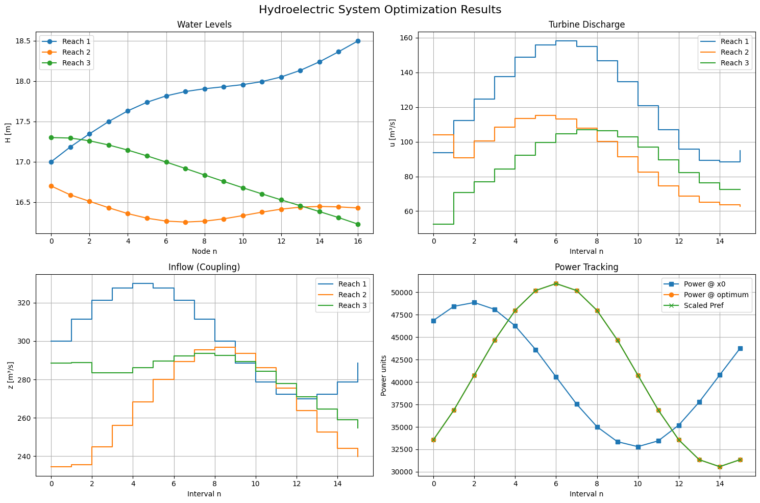
The figure shows the result of a multiple-shooting optimization applied to a three-reach hydroelectric cascade. The time horizon is discretized into 16 intervals, and SciPy’s trust-constr solver is used to find a feasible control sequence that satisfies mass balance, turbine and spillway limits, and Muskingum-style routing dynamics. Each reach integrates its own local ODE, with continuity constraints linking the flows between reaches.
The top-left panel shows the water levels in each reservoir. We observe that upstream reservoirs tend to increase their levels ahead of discharge events, building potential energy before releasing water downstream. The top-right panel shows turbine discharges for each reach. These vary smoothly and are temporally coordinated across the system. The bottom-right panel compares the total generation to a synthetic demand profile, which is generated by a sum of time-shifted sigmoids and normalized to be feasible given turbine capacities. The optimized schedule (orange) tracks this demand closely, while the initial guess (blue) lags behind. The bottom-left panel plots the routed inflows between reaches, which display the expected lag and smoothing effects from Muskingum routing. The interplay between these plots shows how the system anticipates, stores, and routes water to meet time-varying generation targets within physical and operational limits.