Policy Gradient Methods

The previous chapter showed how to handle continuous action spaces in fitted Q-iteration by amortizing action selection with policy networks. Methods like NFQCA, DDPG, TD3, and SAC all learn both a Q-function and a policy, using the Q-function to guide policy improvement. This chapter explores a different approach: optimizing policies directly without maintaining explicit value functions.

Direct policy optimization offers several advantages. First, it naturally handles stochastic policies, which can be essential for partially observable environments or problems requiring explicit exploration. Second, it avoids the detour through value function approximation, which may introduce errors that compound during policy extraction. Third, for problems with simple policy classes but complex value landscapes, directly searching in policy space can be more efficient than searching in value space.

The foundation of policy gradient methods rests on computing gradients of expected returns with respect to policy parameters. This chapter develops the mathematical machinery needed for this computation, starting with general derivative estimation techniques from stochastic optimization, then specializing to reinforcement learning settings, and finally examining variance reduction methods that make these estimators practical.

Derivative Estimation for Stochastic Optimization¶

Consider optimizing an objective that involves an expectation:

For concreteness, consider a simple example where $x \sim \mathcal{N}(\theta,1)$ and $f(x,\theta) = x^2\theta$. The derivative we seek is:

While we can compute this exactly for the Gaussian example, this is often impossible for more general problems. We might then be tempted to approximate our objective using samples:

Then differentiate this approximation:

However, this naive approach ignores that the samples themselves depend on $\theta$. The correct derivative requires the product rule:

While the first term could be numerically integrated using Monte Carlo, the second one cannot as it is not in the form of an expectation.

To transform our objective so that the Monte Carlo estimator for the objective could be differentiated directly while ensuring that the resulting derivative is unbiased, there are two main solutions: a change of measure, or a change of variables.

The Likelihood Ratio Method¶

One solution comes from rewriting our objective using a proposal distribution $q(x)$ that does not depend on $\theta$:

Define the likelihood ratio $\rho(x, q, \theta) \equiv \frac{p(x;\theta)}{q(x)}$, where we treat $q$ as a separate argument. The objective becomes:

When we differentiate $J$, we take the partial derivative with respect to $\theta$ while holding $q$ fixed (since $q$ does not depend on $\theta$):

The partial derivative of $\rho$ with respect to $\theta$ (treating $q$ as fixed) is:

Now fix any reference parameter $\theta_0$ and choose the proposal distribution $q(x) = p(x;\theta_0)$. This is a fixed distribution that does not change as $\theta$ varies. We simply evaluate the family $p(x;\cdot)$ at the specific point $\theta_0$. With this choice, evaluating the gradient at $\theta = \theta_0$ gives $\rho(x, q, \theta_0) = p(x;\theta_0)/p(x;\theta_0) = 1$. The gradient formula becomes:

Since $\theta_0$ is arbitrary, we can drop the subscript and write the score function estimator as:

The Reparameterization Trick¶

An alternative approach eliminates the $\theta$-dependence in the sampling distribution by expressing $x$ through a deterministic transformation of the noise:

Therefore if we want to sample from some target distribution $p(x;\theta)$, we can do so by first sampling from a simple base distribution $q(\epsilon)$ (like a standard normal) and then transforming those samples through a carefully chosen function $g$. If $g(\cdot,\theta)$ is invertible, the change of variables formula tells us how these distributions relate:

For example, if we want to sample from any multivariate Gaussian distributions with covariance matrix $\Sigma$ and mean $\mu$, it suffices to be able to sample from a standard normal noise and compute the linear transformation:

where $\Sigma^{1/2}$ is the matrix square root obtained via Cholesky decomposition. In the univariate case, this transformation is simply:

where $\sigma = \sqrt{\sigma^2}$ is the standard deviation (square root of the variance).

Common Examples of Reparameterization¶

The Truncated Normal Distribution¶

When we need samples constrained to an interval $[a,b]$, we can use the truncated normal distribution. To sample from it, we transform uniform noise through the inverse cumulative distribution function (CDF) of the standard normal:

Here:

• $\Phi(z) = \frac{1}{2}\left[1 + \text{erf}\left(\frac{z}{\sqrt{2}}\right)\right]$ is the CDF of the standard normal distribution

• $\Phi^{-1}$ is its inverse (the quantile function)

• $\text{erf}(z) = \frac{2}{\sqrt{\pi}}\int_0^z e^{-t^2}dt$ is the error function

The resulting samples follow a normal distribution restricted to $[a,b]$, with the density properly normalized over this interval.

The Kumaraswamy Distribution¶

When we need samples in the unit interval [0,1], a natural choice might be the Beta distribution. However, its inverse CDF doesn’t have a closed form. Instead, we can use the Kumaraswamy distribution as a convenient approximation, which allows for a simple reparameterization:

where:

• $\alpha, \beta > 0$ are shape parameters that control the distribution

• $\alpha$ determines the concentration around 0

• $\beta$ determines the concentration around 1

• The distribution is similar to Beta(α,β) but with analytically tractable CDF and inverse CDF

The Kumaraswamy distribution has density:

The Gumbel-Softmax Distribution¶

When sampling from a categorical distribution with probabilities $\{\pi_i\}$, one approach uses $\text{Gumbel}(0,1)$ noise combined with the argmax of log-perturbed probabilities:

This approach, known in machine learning as the Gumbel-Max trick, relies on sampling Gumbel noise from uniform random variables through the transformation $g_i = -\log(-\log(u_i))$ where $u_i \sim \text{Uniform}(0,1)$. To see why this gives us samples from the categorical distribution, consider the probability of selecting category $i$:

Since the difference of two Gumbel random variables follows a logistic distribution, $g_i - g_j \sim \text{Logistic}(0,1)$, and these differences are independent for different $j$ (due to the independence of the original Gumbel variables), we can write:

The last equality requires some additional algebra to show, but follows from the fact that these probabilities must sum to 1 over all $i$.

While we have shown that the Gumbel-Max trick gives us exact samples from a categorical distribution, the argmax operation isn’t differentiable. For stochastic optimization problems of the form:

we need $g$ to be differentiable with respect to $\theta$. This leads us to consider a continuous relaxation where we replace the hard argmax with a temperature-controlled softmax:

As $\tau \to 0$, this approximation approaches the argmax:

The resulting distribution over the probability simplex is called the Gumbel-Softmax (or Concrete) distribution. The temperature parameter $\tau$ controls the discreteness of our samples: smaller values give samples closer to one-hot vectors but with less stable gradients, while larger values give smoother gradients but more diffuse samples.

Numerical Analysis of Gradient Estimators¶

Let us examine the behavior of our three gradient estimators for the stochastic optimization objective:

To get an analytical expression for the derivative, first note that we can factor out $\theta$ to obtain $J(\theta) = \theta\mathbb{E}[x^2]$ where $x \sim \mathcal{N}(\theta,1)$. By definition of the variance, we know that $\text{Var}(x) = \mathbb{E}[x^2] - (\mathbb{E}[x])^2$, which we can rearrange to $\mathbb{E}[x^2] = \text{Var}(x) + (\mathbb{E}[x])^2$. Since $x \sim \mathcal{N}(\theta,1)$, we have $\text{Var}(x) = 1$ and $\mathbb{E}[x] = \theta$, therefore $\mathbb{E}[x^2] = 1 + \theta^2$. This gives us:

Now differentiating with respect to $\theta$ using the product rule yields:

For concreteness, we fix $\theta = 1.0$ and analyze samples drawn using Monte Carlo estimation with batch size 1000 and 1000 independent trials. Evaluating at $\theta = 1$ gives us $\frac{d}{d\theta}J(\theta)\big|_{\theta=1} = 1 + 3(1)^2 = 4$, which serves as our ground truth against which we compare our estimators:

1. First, we consider the naive estimator that incorrectly differentiates the Monte Carlo approximation:

   $$\hat{g}_{\text{naive}}(\theta) = \frac{1}{N}\sum_{i=1}^N x_i^2$$

   (28)

   For $x \sim \mathcal{N}(1,1)$, we have $\mathbb{E}[x^2] = \theta^2 + 1 = 2.0$ and $\mathbb{E}[\hat{g}_{\text{naive}}] = 2.0$. We should therefore expect a bias of about -2 in our experiment.

2. Then we compute the score function estimator:

   $$\hat{g}_{\text{SF}}(\theta) = \frac{1}{N}\sum_{i=1}^N \left[x_i^2\theta(x_i - \theta) + x_i^2\right]$$

   (29)

   This estimator is unbiased with $\mathbb{E}[\hat{g}_{\text{SF}}] = 4$

3. Finally, through the reparameterization $x = \theta + \epsilon$ where $\epsilon \sim \mathcal{N}(0,1)$, we obtain:

   $$\hat{g}_{\text{RT}}(\theta) = \frac{1}{N}\sum_{i=1}^N \left[2\theta(\theta + \epsilon_i) + (\theta + \epsilon_i)^2\right]$$

   (30)

   This estimator is also unbiased with $\mathbb{E}[\hat{g}_{\text{RT}}] = 4$.

Source

%config InlineBackend.figure_format = 'retina'
import jax
import jax.numpy as jnp
import matplotlib.pyplot as plt

# Apply book style
try:
    import scienceplots
    plt.style.use(['science', 'notebook'])
except (ImportError, OSError):
    pass  # Use matplotlib defaults

key = jax.random.PRNGKey(0)

# Define the objective function f(x,θ) = x²θ where x ~ N(θ, 1)
def objective(x, theta):
    return x**2 * theta

# Naive Monte Carlo gradient estimation
@jax.jit
def naive_gradient_batch(key, theta):
    samples = jax.random.normal(key, (1000,)) + theta
    # Use jax.grad on the objective with respect to theta
    grad_fn = jax.grad(lambda t: jnp.mean(objective(samples, t)))
    return grad_fn(theta)

# Score function estimator (REINFORCE)
@jax.jit
def score_function_batch(key, theta):
    samples = jax.random.normal(key, (1000,)) + theta
    # f(x,θ) * ∂logp(x|θ)/∂θ + ∂f(x,θ)/∂θ
    # score function for N(θ,1) is (x-θ)
    score = samples - theta
    return jnp.mean(objective(samples, theta) * score + samples**2)

# Reparameterization gradient
@jax.jit
def reparam_gradient_batch(key, theta):
    eps = jax.random.normal(key, (1000,))
    # Use reparameterization x = θ + ε, ε ~ N(0,1)
    grad_fn = jax.grad(lambda t: jnp.mean(objective(t + eps, t)))
    return grad_fn(theta)

# Run trials
n_trials = 1000
theta = 1.0
true_grad = 1 + 3 * theta**2

keys = jax.random.split(key, n_trials)
naive_estimates = jnp.array([naive_gradient_batch(k, theta) for k in keys])
score_estimates = jnp.array([score_function_batch(k, theta) for k in keys])
reparam_estimates = jnp.array([reparam_gradient_batch(k, theta) for k in keys])

# Create violin plots with individual points
plt.figure(figsize=(12, 6))
data = [naive_estimates, score_estimates, reparam_estimates]
colors = ['#ff9999', '#66b3ff', '#99ff99']

parts = plt.violinplot(data, showextrema=False)
for i, pc in enumerate(parts['bodies']):
    pc.set_facecolor(colors[i])
    pc.set_alpha(0.7)

# Add box plots
plt.boxplot(data, notch=True, showfliers=False)

# Add true gradient line
plt.axhline(y=true_grad, color='r', linestyle='--', label='True Gradient')

plt.xticks([1, 2, 3], ['Naive', 'Score Function', 'Reparam'])
plt.ylabel('Gradient Estimate')
plt.title(f'Gradient Estimators (θ={theta}, true grad={true_grad:.2f})')
plt.grid(True, alpha=0.3)
plt.legend()

# Print statistics
methods = {
    'Naive': naive_estimates,
    'Score Function': score_estimates, 
    'Reparameterization': reparam_estimates
}

for name, estimates in methods.items():
    bias = jnp.mean(estimates) - true_grad
    variance = jnp.var(estimates)
    print(f"\n{name}:")
    print(f"Mean: {jnp.mean(estimates):.6f}")
    print(f"Bias: {bias:.6f}")
    print(f"Variance: {variance:.6f}")
    print(f"MSE: {bias**2 + variance:.6f}")

Naive:
Mean: 2.000417
Bias: -1.999583
Variance: 0.005933
MSE: 4.004266

Score Function:
Mean: 3.996162
Bias: -0.003838
Variance: 0.057295
MSE: 0.057309

Reparameterization:
Mean: 3.999940
Bias: -0.000060
Variance: 0.017459
MSE: 0.017459

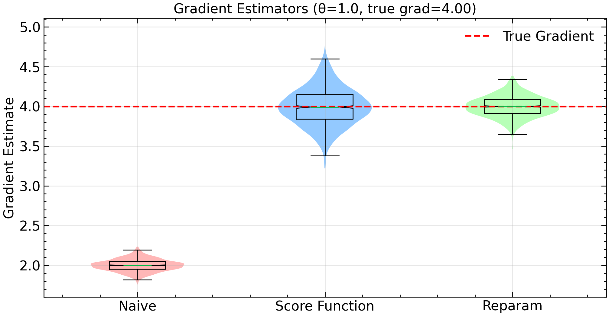
The numerical experiments corroborate our theory. The naive estimator consistently underestimates the true gradient by 2.0, though it maintains a relatively small variance. This systematic bias would make it unsuitable for optimization despite its low variance. The score function estimator corrects this bias but introduces substantial variance. While unbiased, this estimator would require many samples to achieve reliable gradient estimates. Finally, the reparameterization trick achieves a much lower variance while remaining unbiased. While this experiment is for didactic purposes only, it reproduces what is commonly found in practice: that when applicable, the reparameterization estimator tends to perform better than the score function counterpart.

Score Function Methods in Reinforcement Learning¶

The score function estimator from the previous section applies directly to reinforcement learning. Since it requires only the ability to evaluate and differentiate $\log \pi_{\boldsymbol{w}}(a|s)$, it works with any differentiable policy, including discrete action spaces where reparameterization is unavailable. It requires no model of the environment dynamics.

Let $G(\tau) \equiv \sum_{t=0}^T r(s_t, a_t)$ be the sum of undiscounted rewards in a trajectory $\tau$. The stochastic optimization problem we face is to maximize:

where $\tau = (s_0,a_0,s_1,a_1,...)$ is a trajectory and $G(\tau)$ is the total return. Applying the score function estimator, we get:

We have eliminated the need to know the transition probabilities in this estimator since the probability of a trajectory factorizes as:

Therefore, only the policy depends on $\boldsymbol{w}$. When taking the logarithm of this product, we get a sum where all the $\boldsymbol{w}$-independent terms vanish. The final estimator samples trajectories under the distribution $p(\tau; \boldsymbol{w})$ and computes:

This is a direct application of the score function estimator. However, we rarely use this form in practice and instead make several improvements to further reduce the variance.

Leveraging Conditional Independence¶

Given the Markov property of the MDP, rewards $r_k$ for $k < t$ are conditionally independent of action $a_t$ given the history $h_t = (s_0,a_0,...,s_{t-1},a_{t-1},s_t)$. This allows us to only need to consider future rewards when computing policy gradients.

The conditional independence assumption means that the term $\mathbb{E}_{\tau}\left[\sum_{t=0}^T\nabla_{\boldsymbol{w}}\log \pi_{\boldsymbol{w}}(a_t|s_t)\sum_{k=0}^{t-1} r_k \right]$ vanishes. To see this, factor the trajectory distribution as:

We can now re-write a single term of this summation as:

The inner expectation is zero because

The Monte Carlo estimator becomes:

This gives us the REINFORCE algorithm:

The benefit of this estimator compared to the naive one (which would weight each score function by the full trajectory return $G(\tau)$) is that it generally has less variance. This variance reduction arises from the conditional independence structure we exploited: past rewards do not depend on future actions. More formally, this estimator is an instance of a variance reduction technique known as the Extended Conditional Monte Carlo Method.

The Surrogate Loss Perspective¶

The algorithm above computes a gradient estimate $\hat{g}$ explicitly. In practice, implementations using automatic differentiation frameworks take a different approach: they define a surrogate loss whose gradient matches the REINFORCE estimator. For a single trajectory, consider:

where the returns $G_t$ and actions $a_t$ are treated as fixed constants (detached from the computation graph). Taking the gradient with respect to $\boldsymbol{w}$:

Minimizing this surrogate loss via gradient descent yields the same update as maximizing expected return via REINFORCE. The negative sign converts our maximization problem into a minimization suitable for standard optimizers.

This surrogate loss is not the expected return $J(\boldsymbol{w})$ we are trying to maximize. It is a computational device that produces the correct gradient at the current parameter values. Several properties distinguish it from a true loss function:

1. It changes each iteration. The returns $G_t$ come from trajectories sampled under the current policy. After updating $\boldsymbol{w}$, we must collect new trajectories and construct a new surrogate loss.

2. Its value is not meaningful. Unlike supervised learning where the loss measures prediction error, the numerical value of $L_{\text{surrogate}}$ has no direct interpretation. Only its gradient matters.

3. It is valid only locally. The surrogate loss provides the correct gradient only at the parameters used to collect the data. Moving far from those parameters invalidates the gradient estimate.

This perspective explains why policy gradient code often looks different from the pseudocode above. Instead of computing $\hat{g}$ explicitly, implementations define the surrogate loss and call loss.backward():

# Surrogate loss implementation (single trajectory)
log_probs = [policy.log_prob(a_t, s_t) for s_t, a_t in trajectory]
returns = compute_returns(rewards)
surrogate_loss = -sum(lp * G for lp, G in zip(log_probs, returns))
surrogate_loss.backward()  # computes REINFORCE gradient
optimizer.step()

Variance Reduction via Control Variates¶

Recall that the REINFORCE gradient estimator, after leveraging conditional independence, takes the form:

This is a sum over trajectories and timesteps. The gradient contribution at timestep $t$ of trajectory $i$ is:

While unbiased, this estimator suffers from high variance because the return $\sum_{k=t}^T r_k$ can vary significantly across trajectories even for the same state-action pair. The control variate method provides a principled way to reduce this variance.

General Control Variate Theory¶

For a general estimator $Z$ of some quantity $\mu = \mathbb{E}[Z]$, and a control variate $C$ with known expectation $\mathbb{E}[C]=0$, we can construct:

This remains unbiased since $\mathbb{E}[Z_{\text{cv}}] = \mathbb{E}[Z] - \alpha\mathbb{E}[C] = \mathbb{E}[Z]$. The variance is:

The $-2\alpha\text{Cov}(Z,C)$ term is what enables variance reduction. If $Z$ and $C$ are positively correlated, we can choose $\alpha > 0$ to make this term negative and large in magnitude, reducing the overall variance. However, the $\alpha^2\text{Var}(C)$ term grows quadratically with $\alpha$, so if we make $\alpha$ too large, this quadratic term will eventually dominate and the variance will increase rather than decrease. The variance as a function of $\alpha$ is a parabola opening upward, with a unique minimum. Setting $\frac{d}{d\alpha}\text{Var}(Z_{\text{cv}}) = 0$ gives:

This is the coefficient from ordinary least squares regression: we predict the estimator $Z$ using the control variate $C$ as the predictor. Since $\mathbb{E}[C] = 0$, the linear model is $Z \approx \mathbb{E}[Z] + \alpha^* C$, where $\alpha^*$ is the OLS slope coefficient. The control variate estimator $Z_{\text{cv}} = Z - \alpha^* C$ computes the residual: the part of $Z$ that cannot be explained by $C$.

Substituting $\alpha^*$ into the variance formula yields:

where $R^2 = \frac{[\text{Cov}(Z,C)]^2}{\text{Var}(Z)\text{Var}(C)}$ is the coefficient of determination from regressing $Z$ on $C$. The variance reduction is $R^2 \text{Var}(Z)$: the better $C$ predicts $Z$, the more variance we eliminate.

Application to REINFORCE¶

In the reinforcement learning setting, our REINFORCE gradient estimator is a sum over timesteps: $\sum_{t=0}^T Z_t$ where each $Z_t$ represents the gradient contribution at timestep $t$. We apply control variates separately to each term. Since $\text{Var}(\sum_t Z_t) = \sum_t \text{Var}(Z_t) + \sum_{t \neq s} \text{Cov}(Z_t, Z_s)$, reducing the variance of each $Z_t$ reduces the total variance, though we do not explicitly address the cross-timestep covariance terms.

For a given trajectory at state $s_t$, the gradient contribution at time $t$ is:

This is the product of the score function $\nabla_{\boldsymbol{w}}\log \pi_{\boldsymbol{w}}(a_t|s_t)$ and the return-to-go $\sum_{k=t}^T r_k$. We can subtract any state-dependent function $b(s_t)$ from the return without introducing bias, as long as $b(s_t)$ does not depend on $a_t$. This is because:

where the last equality follows from the score function identity (38).

We can now define our control variate as:

where $b(s_t)$ is a baseline function that depends only on the state. This satisfies $\mathbb{E}[C_t|s_t] = 0$. Our control variate estimator becomes:

The optimal baseline $b^*(s_t)$ minimizes the variance. To find it, consider the scalar parameter case for simplicity. Write $g(a_t) \equiv \nabla_w \log \pi_w(a_t|s_t)$ and $G_t = \sum_{k=t}^T r_k$. We want to minimize:

Since the mean does not depend on $b$, minimizing the variance is equivalent to minimizing the second moment $\mathbb{E}[g(a_t)^2(G_t - b)^2|s_t]$. Expanding and taking the derivative with respect to $b$ gives:

For vector-valued parameters $\boldsymbol{w}$, we minimize a scalar proxy such as the trace of the covariance matrix, which yields the same formula with $\|\nabla_{\boldsymbol{w}}\log \pi_{\boldsymbol{w}}(a_t|s_t)\|^2$ in place of $g(a_t)^2$:

This is the exact optimal baseline: a weighted average of returns where the weights are the squared norms of the score function. In practice, we treat the squared norm as roughly constant across actions at a given state, which leads to the simpler and widely used choice:

With this approximation, the variance-reduced gradient contribution at timestep $t$ becomes:

The term in parentheses is exactly the advantage function: $A^{\pi_{\boldsymbol{w}}}(s_t, a_t) = q^{\pi_{\boldsymbol{w}}}(s_t, a_t) - v^{\pi_{\boldsymbol{w}}}(s_t)$, where the Q-function is approximated by the Monte Carlo return $\sum_{k=t}^T r_k$. The full gradient estimate for a trajectory is then the sum over all timesteps:

In practice, we do not have access to the true value function and must learn it. Unlike the methods in the amortization chapter, where we learned value functions to approximate the optimal Q-function, here our goal is policy evaluation: estimating the value of the current policy $\pi_{\boldsymbol{w}}$. The same function approximation techniques apply, but we target $v^{\pi_{\boldsymbol{w}}}$ rather than $v^*$. The simplest approach is to regress from states to Monte Carlo returns, learning what Williams (1992) called a “baseline”:

When implementing this algorithm nowadays, we always use mini-batching to make full use of our GPUs. Therefore, a more representative variant for this algorithm would be:

The value function is trained by regressing states directly to their sampled Monte Carlo returns $G$. Advantage normalization (step 2.5) is not part of the optimal baseline derivation but improves optimization in practice and is standard in modern implementations.

Generalized Advantage Estimation¶

The baseline construction gave us a gradient estimator of the form:

where $G_t = \sum_{k=t}^T r_k$ is the Monte Carlo return from time $t$. For each visited state-action pair $(s_t, a_t)$, the term in parentheses

is a Monte Carlo estimate of the advantage $A^{\pi}(s_t, a_t) = q^{\pi}(s_t, a_t) - v^{\pi}(s_t)$. If the baseline equals the true value function, $v = v^{\pi}$, then $\mathbb{E}[\widehat{A}_t^{\text{MC}} | s_t, a_t] = A^{\pi}(s_t, a_t)$, so this estimator is unbiased.

However, as an estimator it has two limitations. First, it has high variance because $G_t$ depends on all future rewards. Second, it uses the value function only as a baseline, not as a predictor of long-term returns. We essentially discard the information in $v(s_{t+1}), v(s_{t+2}), \ldots$

GAE addresses these issues by constructing a family of estimators that interpolate between pure Monte Carlo and pure bootstrapping. A parameter $\lambda$ controls the bias-variance tradeoff.

Decomposing the Monte Carlo Advantage¶

Fix a value function $v(s)$ (not necessarily equal to $v^{\pi}$) and define the one-step residual:

Start from the Monte Carlo advantage and add and subtract $\gamma v(s_{t+1})$:

Applying this decomposition recursively yields:

The Monte Carlo advantage is exactly the discounted sum of future residuals. This is an algebraic identity, not an approximation.

The sequence $\{\delta_{t+l}\}_{l \geq 0}$ provides incremental corrections to the value function as we move forward in time. The term $\delta_t$ depends only on $(s_t, a_t, s_{t+1})$; $\delta_{t+1}$ depends on $(s_{t+1}, a_{t+1}, s_{t+2})$, and so on. As $l$ increases, the corrections become more noisy (they depend on more random outcomes) and more sensitive to errors in the value function at later states. Although the full sum is unbiased when $v = v^{\pi}$, it can have high variance and can be badly affected by approximation error in $v$.

GAE as a Shrinkage Estimator¶

The decomposition above suggests a family of estimators that downweight residuals farther in the future. Let $\lambda \in [0,1]$ and define:

This is the generalized advantage estimator $A_t^{\text{GAE}(\gamma,\lambda)}$.

Two special cases illustrate the extremes. When $\lambda = 1$, we recover the Monte Carlo advantage:

When $\lambda = 0$, we keep only the immediate residual:

Intermediate values $0 < \lambda < 1$ interpolate between these extremes. The influence of $\delta_{t+l}$ decays geometrically as $(\gamma\lambda)^l$. The parameter $\lambda$ acts as a shrinkage parameter: small $\lambda$ shrinks the estimator toward the one-step residual; large $\lambda$ allows the estimator to behave more like the Monte Carlo advantage.

If $v = v^{\pi}$ is the true value function, then $\mathbb{E}[\delta_t | s_t, a_t] = A^{\pi}(s_t, a_t)$ and $\mathbb{E}[\delta_{t+l} | s_t, a_t] = 0$ for $l \geq 1$. In this case:

for all $\lambda \in [0,1]$. When the value function is exact, GAE is unbiased regardless of $\lambda$; changing $\lambda$ only affects variance.

In practice, we approximate $v^{\pi}$ with a function approximator, and the residuals $\delta_{t+l}$ inherit approximation error. Distant residuals involve multiple applications of the approximate value function and are more contaminated by modeling error. Downweighting them (choosing $\lambda < 1$) introduces bias but can reduce variance and limit the impact of those errors.

Mixture of Multi-Step Estimators¶

Another perspective on GAE comes from multi-step returns. Define the $k$-step return from time $t$:

and the corresponding $k$-step advantage estimator $A_t^{(k)} = G_t^{(k)} - v(s_t)$. Each $A_t^{(k)}$ uses $k$ rewards before bootstrapping; larger $k$ means more variance but less bootstrapping error.

The GAE estimator can be written as a geometric mixture:

GAE is a weighted average of the $k$-step advantage estimators, with shorter horizons weighted more heavily when $\lambda$ is small.

Using GAE in the Policy Gradient¶

Once we choose $\lambda$, we plug $A_t^{\lambda}$ in place of $G_t - v(s_t)$ in the policy gradient estimator:

We still use a control variate to reduce variance (the baseline $v$), but now we construct the advantage target by smoothing the sequence of residuals $\{\delta_t\}$ with a geometrically decaying kernel.

For the value function, it is convenient to define the $\lambda$-return:

When $\lambda = 1$, $G_t^{\lambda}$ reduces to the Monte Carlo return; when $\lambda = 0$, it becomes the one-step bootstrapped target $r_t + \gamma v(s_{t+1})$.

When $\lambda = 1$, this reduces (up to advantage normalization) to the Monte Carlo baseline algorithm earlier in the chapter. When $\lambda = 0$, advantages become the one-step residuals $\delta_t$, and the $\lambda$-returns reduce to standard one-step bootstrapped targets.

Actor-Critic as the $\lambda = 0$ Limit¶

The case $\lambda = 0$ is particularly simple. The advantage becomes:

and the policy update reduces to:

while the value update becomes a standard one-step regression toward $r_t + \gamma v(s_{t+1})$. This gives the online actor-critic algorithm:

This algorithm was derived by Sutton in his 1984 thesis as an “adaptive heuristic” for temporal credit assignment. In the language of this chapter, it is the $\lambda = 0$ member of the GAE family: it uses the most local residual $\delta_t$ as both the target for the value function and the advantage estimate for the policy gradient.

Likelihood Ratio Methods in Reinforcement Learning¶

The score function estimator from the previous section is a special case of the likelihood ratio method where the proposal distribution equals the target distribution. We now consider the general case where they differ.

Recall the likelihood ratio gradient estimator from the beginning of this chapter. For objective $J(\theta) = \mathbb{E}_{x \sim p(x;\theta)}[f(x)]$ and any proposal distribution $q(x)$:

where $\rho(x; q, \theta) = \frac{p(x;\theta)}{q(x)}$ is the likelihood ratio. The partial derivative $\frac{\partial \rho}{\partial \theta} = \rho \nabla_\theta \log p$ holds because $x$ is treated as fixed, having been sampled from $q$, which does not depend on $\theta$.

In reinforcement learning, let $x = \tau$ be a trajectory, $f(\tau) = G(\tau)$ the return, $p(\tau;\boldsymbol{w})$ the trajectory distribution under policy $\pi_{\boldsymbol{w}}$, and $q(\tau)$ the trajectory distribution under some other policy $\pi_q$. The gradient becomes: