Fitted Q-Iteration Methods

The previous chapter established the theoretical foundations of simulation-based approximate dynamic programming: Monte Carlo integration for evaluating expectations, Q-functions for efficient action selection, and techniques for mitigating overestimation bias. Those developments assumed we could sample freely from transition distributions and choose optimization parameters without constraint. This chapter develops a unified framework for fitted Q-iteration algorithms that spans both offline and online settings. We begin with batch algorithms that learn from fixed datasets, then show how the same template generates online methods like DQN through systematic variations in data collection, optimization strategy, and function approximation.

Design Choices in FQI Methods¶

All FQI methods share the same two-level structure built on three core ingredients: a buffer $\mathcal{B}_t$ of transitions inducing an empirical distribution $\hat{P}_{\mathcal{B}_t}$, a target function $g$ that computes regression targets from the current Q-function, and an optimization procedure to fit the Q-function to the resulting targets. At iteration $n$, the outer loop constructs targets from individual transitions using the target function: for each transition $(s_i, a_i, r_i, s'_i)$, we compute $y_i^{(n)} = g(s_i, a_i, r_i, s'_i; \boldsymbol{\theta}_n)$ where typically $g(s,a,r,s'; \boldsymbol{\theta}) = r + \gamma \max_{a'} q(s',a'; \boldsymbol{\theta})$. The inner loop solves the regression problem $\min_{\boldsymbol{\theta}} \mathbb{E}_{((s,a),y) \sim \hat{P}_n^{\text{fit}}}[\ell(q(s, a; \boldsymbol{\theta}), y)]$ to find parameters that match these targets. We can write this abstractly as:

The fit operation minimizes the regression loss using $K$ optimization steps (gradient descent for neural networks, tree construction for ensembles, matrix inversion for linear models) starting from initialization $\boldsymbol{\theta}_{\text{init}}$. Standard supervised learning uses random initialization ($\boldsymbol{\theta}_{\text{init}} = \boldsymbol{\theta}_0$) and runs to convergence ($K = \infty$). Reinforcement learning algorithms vary these choices: warm starting from the previous iteration ($\boldsymbol{\theta}_{\text{init}} = \boldsymbol{\theta}^{(n)}$), partial optimization ($K \in \{10, \ldots, 100\}$), or single-step updates ($K=1$).

The buffer $\mathcal{B}_t$ may stay fixed (batch setting) or change (online setting), but the targets always change because they depend on the evolving target function $g(\cdot; \boldsymbol{\theta}_n)$. In practice, we typically have one observed next state per transition, giving $g(s_i, a_i, r_i, s'_i; \boldsymbol{\theta}) = r_i + \gamma \max_{a'} q(s'_i, a'; \boldsymbol{\theta})$ for transition tuples $(s_i, a_i, r_i, s'_i)$.

This template provides a blueprint for instantiating concrete algorithms. Six design axes generate algorithmic diversity: the function approximator (trees, neural networks, linear models), the Bellman operator (hard max vs smooth logsumexp, discussed in the regularized MDP chapter), the inner optimization strategy (full convergence, $K$ steps, or single step), the initialization scheme (cold vs warm start), the data collection mechanism (offline, online, replay buffer), and bias mitigation approaches (none, double Q-learning, learned correction). While individual algorithms include additional refinements, these axes capture the primary sources of variation. The table below shows how several well-known methods instantiate this template:

This table omits continuous action methods (NFQCA, DDPG, SAC), which introduce an additional design dimension. We address those in the continuous action chapter. The initialization choice becomes particularly important when moving from batch to online algorithms.

Plug-In Approximation with Empirical Distributions¶

The exact Bellman operator involves expectations under the true transition law (combined with the behavior policy), which we denote abstractly by $P$ over transitions $\tau = (s,a,r,s')$:

In fitted Q-iteration we never see $P$ directly. Instead, we collect a finite set of transitions in a buffer $\mathcal{B}_t = \{\tau_1,\dots,\tau_{|\mathcal{B}_t|}\}$ and work with the empirical distribution

where $\delta_\tau$ denotes a Dirac delta (point mass) centered at transition $\tau$. Each $\delta_\tau$ is a probability distribution that places mass 1 at the single point $\tau$ and mass 0 everywhere else. The sum creates a mixture distribution: a uniform distribution over the finite set of observed transitions. Sampling from $\hat{P}_{\mathcal{B}_t}$ means picking one transition uniformly at random from the buffer.

For any integrand $g(\tau)$ (loss, TD error, gradient term), expectations under $P$ are approximated by expectations under $\hat{P}_{\mathcal{B}_t}$ using the sample average estimator:

This is exactly the sample average estimator from the Monte Carlo chapter, applied now to transitions. Conceptually, fitted Q-iteration performs plug-in approximate dynamic programming. The plug-in principle is a general approach from statistics: when an algorithm requires an unknown population quantity, substitute its sample-based estimator. Here, we replace the unknown transition law $P$ with the empirical distribution $\hat{P}_{\mathcal{B}_t}$ and run value iteration using this empirical Bellman operator:

From a computational viewpoint, we could describe all of this using sample averages and mini-batch gradients. The empirical distribution notation provides three benefits. First, it unifies offline and online algorithms: both perform value iteration under an empirical law $\hat{P}_{\mathcal{B}_t}$, differing only in whether $\mathcal{B}_t$ remains fixed or evolves. Second, it shows that methods like DQN perform stochastic optimization of a sample average approximation objective $\mathbb{E}_{\tau \sim \hat{P}_{\mathcal{B}_t}}[\ell(\cdot)]$, not some ad hoc non-stationary procedure. Third, it cleanly separates two sources of approximation that we will examine shortly: statistical bootstrap (resampling from $\hat{P}_{\mathcal{B}_t}$) versus temporal-difference bootstrap (using estimated values in targets).

Data, Buffers, and the Unified Template¶

Fitted Q-iteration is built around three ingredients at any time $t$:

1. A replay buffer $\mathcal{B}_t$ containing transitions, inducing an empirical distribution $\hat{P}_{\mathcal{B}_t}$

2. A target function $g(s,a,r,s'; \boldsymbol{\theta}) : \mathcal{S} \times \mathcal{A} \times \mathbb{R} \times \mathcal{S} \times \Theta \mapsto \mathbb{R}$ that computes regression targets for individual transitions. Unlike the Bellman operator $\mathcal{T}$ which acts on function spaces, $g$ operates on transition tuples with parameters $\boldsymbol{\theta}$ (after the semicolon) specifying the current Q-function. Typically $g(s,a,r,s'; \boldsymbol{\theta}) = r + \gamma \max_{a'} q(s',a'; \boldsymbol{\theta})$ (hard max) or uses the smooth logsumexp operator.

3. A loss function $\ell$ and optimization budget (replay ratio, number of gradient steps)

Pushing transitions through the target function transforms $\hat{P}_{\mathcal{B}_t}$ into a regression distribution $\hat{P}_t^{\text{fit}}$ over pairs $((s,a), y)$, as described in the notation remark above. The inner loop minimizes the empirical risk $\mathbb{E}_{((s,a),y)\sim \hat{P}_t^{\text{fit}}} [\ell(q(s,a;\boldsymbol{\theta}), y)]$ via stochastic gradient descent on mini-batches.

Different algorithms correspond to different ways of evolving the buffer $\mathcal{B}_t$ and different replay ratios:

• Offline FQI. We start from a fixed dataset $\mathcal{D}$ and never collect new data. The buffer is constant, $\mathcal{B}_t \equiv \mathcal{D}$ and $\hat{P}_{\mathcal{B}_t} \equiv \hat{P}_{\mathcal{D}}$, and only the target function $g(\cdot; \boldsymbol{\theta}_t)$ changes as the Q-function evolves.

• Replay (DQN-style). The buffer is a circular buffer of fixed capacity $B$. At each interaction step we append the new transition and, if the buffer is full, drop the oldest one: $\mathcal{B}_t = \{\tau_{t-B+1},\ldots,\tau_t\}$ and $\hat{P}_{\mathcal{B}_t} = \frac{1}{|\mathcal{B}_t|} \sum_{\tau \in \mathcal{B}_t} \delta_{\tau}$. The empirical distribution slides forward through time, but at each update we still sample uniformly from the current buffer.

• Fully online Q-learning. Tabular Q-learning is the degenerate case with buffer size $B=1$: we only keep the most recent transition. Then $\hat{P}_{\mathcal{B}_t}$ is supported on a single point and each update uses that one sample once.

The replay ratio (optimization steps per environment transition) quantifies data reuse:

where $K$ is the number of gradient steps per outer iteration. Large replay ratios reuse the same empirical distribution $\hat{P}_{\mathcal{B}_t}$ many times, implementing sample average approximation (offline FQI). Small replay ratios use each sample once, implementing stochastic approximation (online Q-learning). Higher replay ratios reduce variance of estimates under $\hat{P}_{\mathcal{B}_t}$ but risk overfitting to the idiosyncrasies of the current empirical law, especially when it reflects outdated policies or narrow coverage.

Batch Algorithms: Ernst’s FQI and NFQI¶

We begin with the simplest case from the buffer perspective. We are given a fixed transition dataset $\mathcal{D} = \{(s_i,a_i,r_i,s'_i)\}_{i=1}^N$ and never collect new data. The replay buffer is frozen:

so the only thing that changes across iterations is the target function $g(\cdot; \boldsymbol{\theta}_n)$ induced by the current Q-function. Every outer iteration of FQI samples from the same empirical distribution $\hat{P}_{\mathcal{D}}$ but pushes it through a new target function, producing a new regression distribution $\hat{P}_n^{\text{fit}}$.

At each outer iteration $n$, we construct the input set $X^{(n)} = \{(s_i, a_i)\}_{i=1}^N$ from the same transitions (the state-action pairs remain fixed), compute targets $y_i^{(n)} = g(s_i, a_i, r_i, s'_i; \boldsymbol{\theta}^{(n)}) = r_i + \gamma \max_{a'} q(s'_i, a'; \boldsymbol{\theta}^{(n)})$ using the current Q-function, and solve the regression problem $\boldsymbol{\theta}^{(n+1)} \leftarrow \texttt{fit}(X^{(n)}, y^{(n)}, \boldsymbol{\theta}_{\text{init}}, K)$. The buffer $\mathcal{B}_t = \mathcal{D}$ never changes, but the targets change at every iteration because they depend on the evolving target function $g(\cdot; \boldsymbol{\theta}_n)$. Each transition $(s_i, a_i, r_i, s'_i)$ provides a single Monte Carlo sample $s'_i$ for evaluating the Bellman operator at $(s_i, a_i)$, giving us $\widehat{\Bellman}_1 q$ with $N=1$.

The following algorithm is simply approximate value iteration where expectations under the transition kernel $P$ are replaced by expectations under the fixed empirical distribution $\hat{P}_{\mathcal{D}}$:

The fit operation in line 10 abstracts the inner optimization loop that minimizes $\sum_{i=1}^N \ell(q(s_i, a_i; \boldsymbol{\theta}), y_i^{(n)})$. This line encodes the algorithmic choice of which function approximator to use and how to optimize it. The initialization $\boldsymbol{\theta}_{\text{init}}$ and number of optimization steps $K$ control whether we use cold or warm starting and whether we optimize to convergence or perform partial updates.

Fitted Q-Iteration (FQI): Ernst et al. Ernst et al. (2005) instantiate this template with extremely randomized trees (extra trees), an ensemble method that partitions the state-action space into regions with piecewise constant Q-values. The fit operation trains the ensemble until completion using the tree construction algorithm. Trees handle high-dimensional inputs naturally and the ensemble reduces overfitting. FQI uses cold start initialization: $\boldsymbol{\theta}_{\text{init}} = \boldsymbol{\theta}_0$ (randomly initialized) at every iteration, since trees don’t naturally support incremental refinement. The loss $\ell$ is squared error. This method demonstrated that batch reinforcement learning could work with complex function approximators on continuous-state problems.

Neural Fitted Q-Iteration (NFQI): Riedmiller Riedmiller (2005) replaces the tree ensemble with a neural network $q(s,a; \boldsymbol{\theta})$, providing smooth interpolation across the state-action space. The fit operation runs gradient-based optimization (RProp, chosen for its insensitivity to hyperparameter choices) to convergence: train the network until the loss stops decreasing (multiple epochs through the full dataset $\mathcal{D}$), corresponding to $K=\infty$ in our framework. NFQI uses warm start initialization: $\boldsymbol{\theta}_{\text{init}} = \boldsymbol{\theta}_n$ at iteration $n$, meaning the network continues learning from the previous iteration’s weights rather than resetting. This ensures the network accurately represents the projected Bellman operator before moving to the next outer iteration. For episodic tasks with goal and forbidden regions, Riedmiller uses modified target computations (detailed below).

From Nested to Flattened Q-Iteration¶

Fitted Q-iteration has an inherently nested structure: an outer loop performs approximate value iteration by computing Bellman targets, and an inner loop performs regression by fitting the function approximator to those targets. This nested structure shows that FQI is approximate dynamic programming with function approximation, distinct from supervised learning with changing targets.

When the inner loop uses gradient descent for $K$ steps, we have:

This is a sequence of updates $\boldsymbol{\theta}_n^{(k+1)} = \boldsymbol{\theta}_n^{(k)} - \alpha \nabla_{\boldsymbol{\theta}} \mathcal{L}(\boldsymbol{\theta}_n^{(k)}; \mathcal{D}_n^{\text{fit}})$ for $k = 0, \ldots, K-1$ starting from $\boldsymbol{\theta}_n^{(0)} = \boldsymbol{\theta}_n$. Since these inner updates are themselves a loop, we can algebraically rewrite the nested loops as a single flattened loop. This flattening is purely representational. The algorithm remains approximate value iteration, but the presentation obscures the conceptual structure.

In the flattened form, the parameters used for computing targets are called the target network $\boldsymbol{\theta}_{\text{target}}$, which corresponds to $\boldsymbol{\theta}_n$ in the nested form. The target network gets updated every $K$ steps, marking the boundaries between outer iterations.

In contrast, the parameters being actively trained via gradient descent at each step are called the online network $\boldsymbol{\theta}_t$. In the nested view, these correspond to $\boldsymbol{\theta}_n^{(k)}$ within the inner loop. The term “online” here refers to the fact that these parameters are continuously updated at each gradient step, not that data must be collected online. The distinction is between the actively-training parameters ($\boldsymbol{\theta}_t$) and the frozen parameters used for target computation ($\boldsymbol{\theta}_{\text{target}}$).

The online/target terminology is standard in the deep RL community. Many modern algorithms, especially those that collect data online like DQN, are presented in flattened form. This can make them appear different from batch methods when they are the same template with different design choices.

Tree ensemble methods like random forests or extra trees have no continuous parameter space and no gradient-based optimization. The fit operation builds the entire tree structure in one pass. There’s no sequence of incremental updates to unfold into a single loop. Ernst’s FQI Ernst et al. (2005) retains the explicit nested structure with cold start initialization at each outer iteration, while neural methods can be flattened.

Making the Nested Structure Explicit¶

To see how flattening works, we first make the nested structure completely explicit by expanding the fit operation to show the inner gradient descent loop. In terms of the buffer notation, the inner loop approximately minimizes the empirical risk:

induced by the fixed buffer $\mathcal{B}_n = \mathcal{D}$ and target function $g(\cdot; \boldsymbol{\theta}_n)$. Starting from the generic batch FQI template (Algorithm Algorithm 1), we replace the abstract fit call with explicit gradient updates:

This makes the two-level structure completely transparent. The outer loop (indexed by $n$) computes targets $y_{s,a} = r + \gamma \max_{a'} q(s',a'; \boldsymbol{\theta}_n)$ using the parameters $\boldsymbol{\theta}_n$ from the end of the previous outer iteration. These targets remain fixed throughout the entire inner loop. The inner loop (indexed by $k$) performs $K$ gradient steps to fit $q(s,a; \boldsymbol{\theta})$ to the regression dataset $\mathcal{D}_n^{\text{fit}} = \{((s_i, a_i), y_i)\}$, warm starting from $\boldsymbol{\theta}_n$ (the parameters that computed the targets). After $K$ steps, the inner loop produces $\boldsymbol{\theta}_{n+1} = \boldsymbol{\theta}_n^{(K)}$, which becomes the starting point for the next outer iteration.

The notation $\boldsymbol{\theta}_n^{(k)}$ indicates that we are at inner step $k$ within outer iteration $n$. The targets depend only on $\boldsymbol{\theta}_n = \boldsymbol{\theta}_n^{(0)}$, not on the intermediate inner iterates $\boldsymbol{\theta}_n^{(k)}$ for $k > 0$.

Flattening into a Single Loop¶

We can now flatten the nested structure by treating all gradient steps uniformly and using a global step counter $t$ instead of separate outer/inner counters. We introduce a target network $\boldsymbol{\theta}_{\text{target}}$ that holds the parameters used for computing targets. This target network gets updated every $K$ steps, which marks what would have been the boundary between outer iterations. The transformation works as follows: we replace the outer counter $n$ and inner counter $k$ with a single counter $t$, where $t = nK + k$. When $n$ advances from $n$ to $n+1$, this corresponds to $K$ steps of $t$: from $t = nK$ to $t = (n+1)K$. The target network $\boldsymbol{\theta}_{\text{target}}$ equals $\boldsymbol{\theta}_n$ throughout outer iteration $n$ and gets updated via $\boldsymbol{\theta}_{\text{target}} \leftarrow \boldsymbol{\theta}_t$ every $K$ steps (when $t \bmod K = 0$). Parameters that were $\boldsymbol{\theta}_n^{(k)}$ in nested form become $\boldsymbol{\theta}_t$ in flattened form.

This transformation is purely algebraic. No algorithmic behavior changes, only the presentation:

At step $t$, we have $n = \lfloor t/K \rfloor$ (outer iteration) and $k = t \bmod K$ (position within inner loop). The target network $\boldsymbol{\theta}_{\text{target}}$ equals $\boldsymbol{\theta}_n$ throughout the $K$ steps from $t = nK$ to $t = (n+1)K - 1$, then gets updated to $\boldsymbol{\theta}_{n+1}$ at $t = (n+1)K$. The parameters $\boldsymbol{\theta}_t$ correspond to $\boldsymbol{\theta}_n^{(k)}$ in the nested form. The flattening reindexes the iteration structure: with $K=10$, outer iteration $n=3$, inner step $k=7$ becomes global step $t = 3 \cdot 10 + 7 = 37$.

Flattening replaces the pair $(n,k)$ by a single global step index $t$, but the underlying empirical distribution $\hat{P}_{\mathcal{D}}$ remains the same. We still sample from the fixed offline dataset throughout.

The target network arises directly from flattening the nested FQI structure. When DQN is presented with a target network that updates every $K$ steps, this is approximate value iteration in flattened form. The algorithm still performs outer loop (value iteration) and inner loop (regression), but the presentation obscures this structure. The periodic target updates mark the boundaries between outer iterations. DQN is batch approximate DP in flattened form, using online data collection with a replay buffer.

Smooth Target Updates via Exponential Moving Average¶

An alternative to periodic hard updates is exponential moving average (EMA) (also called Polyak averaging), which updates the target network smoothly at every step rather than synchronizing it every $K$ steps:

With EMA updates, the target network slowly tracks the online network instead of making discrete jumps. For small $\tau$ (typically $\tau \in [0.001, 0.01]$), the target lags behind the online network by roughly $1/\tau$ steps. This provides smoother learning dynamics and avoids the discontinuous changes in targets that occur with periodic hard updates. The EMA approach became popular with DDPG Lillicrap et al. (2015) for continuous control and is now standard in algorithms like TD3 Fujimoto et al. (2018) and SAC Haarnoja et al. (2018).

Online Algorithms: DQN and Extensions¶

We now keep the same fitted Q-iteration template but allow the buffer $\mathcal{B}_t$ and its empirical distribution $\hat{P}_{\mathcal{B}_t}$ to evolve while we learn. Instead of repeatedly sampling from a fixed $\hat{P}_{\mathcal{D}}$, we collect new transitions during learning and store them in a circular replay buffer.

Note that “online” here takes on a second meaning: we collect data online (interacting with the environment) while also maintaining the online network (actively-updated parameters $\boldsymbol{\theta}_t$) and target network (frozen parameters $\boldsymbol{\theta}_{\text{target}}$) distinction from the flattened FQI structure. The online network now plays a dual role: it is both the parameters being trained and the policy used to collect new data for the buffer.

Deep Q-Network (DQN) instantiates the online template with moderate choices along the design axes: buffer capacity $B \approx 10^6$, mini-batch size $b \approx 32$, and target network update frequency $K \approx 10^4$. DQN is not an ad hoc collection of tricks. It is fitted Q-iteration in flattened form (as developed in the nested-to-flattened transformation earlier) with an evolving buffer $\mathcal{B}_t$ and low replay ratio.

Deep Q-Network (DQN)¶

Deep Q-Network (DQN) maintains a circular replay buffer of capacity $B$ (typically $B \approx 10^6$). At each environment step, we store the new transition and sample a mini-batch of size $b$ from the buffer for training. This increases the replay ratio, reducing gradient variance at the cost of older, potentially off-policy data.

DQN uses two copies of the Q-network parameters:

• The online network $\boldsymbol{\theta}_t$: actively updated at each gradient step (corresponds to $\boldsymbol{\theta}_n^{(k)}$ in the nested view). It serves a dual role: (1) the policy for collecting new data via $\varepsilon$-greedy action selection, and (2) the parameters being trained.

• The target network $\boldsymbol{\theta}_{\text{target}}$: frozen parameters updated every $K$ steps (corresponds to $\boldsymbol{\theta}_n$ in the nested view). Used only for computing Bellman targets.

As shown in the nested-to-flattened section, the target network is not a stabilization trick but the natural consequence of periodic outer-iteration boundaries in flattened FQI. The target network keeps targets fixed for $K$ gradient steps, which corresponds to the inner loop in the nested view:

Double Deep Q-Network (Double DQN)¶

Double DQN addresses overestimation bias by decoupling action selection from evaluation. Instead of using the target network for both purposes (as DQN does), Double DQN uses the online network (currently-training parameters $\boldsymbol{\theta}_t$) to select which action looks best, then uses the target network (frozen parameters $\boldsymbol{\theta}_{\text{target}}$) to evaluate that action:

Double DQN leaves $\mathcal{B}_t$ and $\hat{P}_{\mathcal{B}_t}$ unchanged and modifies only the target function $g$ by decoupling action selection (online network) from evaluation (target network). Compare the two approaches:

• DQN (blue): Uses the target network $\boldsymbol{\theta}_{\text{target}}$ for BOTH selecting which action is best AND evaluating it: $\max_{a'} q(s',a'; \boldsymbol{\theta}_{\text{target}})$ implicitly finds $a^* = \arg\max_{a'} q(s',a'; \boldsymbol{\theta}_{\text{target}})$ and then evaluates $q(s',a^*; \boldsymbol{\theta}_{\text{target}})$

• Double DQN (red + green): Uses the online network $\boldsymbol{\theta}_t$ to select $a^* = \arg\max_{a'} q(s',a'; \boldsymbol{\theta}_t)$, then uses the target network $\boldsymbol{\theta}_{\text{target}}$ to evaluate $q(s',a^*; \boldsymbol{\theta}_{\text{target}})$

This decoupling prevents overestimation bias because the noise in action selection (from the online network) is independent of the noise in action evaluation (from the target network). Recall that the online network represents the currently-training parameters being updated at each gradient step, while the target network represents the frozen parameters used for computing targets. By using different parameters for selection versus evaluation, we break the correlation that leads to systematic overestimation in the standard max operator.

Q-Learning: The Limiting Case¶

DQN and Double DQN use moderate settings: $B \approx 10^6$, $K \approx 10^4$, mini-batch size $b \approx 32$. We can ask: what happens at the extreme where we minimize buffer capacity, eliminate replay, and update targets every step? This limiting case gives classical Q-learning Watkins (1989): buffer capacity $B=1$, target network frequency $K=1$, and mini-batch size $b=1$.

In the buffer perspective, Q-learning has $\mathcal{B}_t = \{(s_t, a_t, r_t, s'_t)\}$ with $|\mathcal{B}_t | = 1$. The empirical distribution $\hat{P}_{\mathcal{B}_t}$ collapses to a Dirac mass at the current transition. We use each transition exactly once then discard it. There is no separate target network: the parameters used for computing targets are immediately updated after each step ($K=1$, or equivalently $\tau=1$ in EMA). This makes Q-learning a stochastic approximation method with replay ratio 1.

Stochastic approximation is a general framework for solving equations of the form $\mathbb{E}[h(X; \boldsymbol{\theta})] = 0$ using noisy samples, without computing expectations explicitly. The classic example is root-finding: given function $f(\boldsymbol{\theta}; Z)$ whose expectation $\mathbb{E}[f(\boldsymbol{\theta}; Z)] = F(\boldsymbol{\theta})$ we want to solve $F(\boldsymbol{\theta}) = 0$, the Robbins-Monro procedure updates:

using noisy samples $Z_t$ without ever computing $F(\boldsymbol{\theta})$ or its Jacobian. This is analogous to Newton’s method in the deterministic case, but replaces exact gradients with stochastic estimates and avoids computing or inverting the Jacobian. Under diminishing step sizes ($\alpha_t \to 0$, $\sum_t \alpha_t = \infty$), the iterates converge to solutions of $F(\boldsymbol{\theta}) = 0$.

Q-learning fits this framework by solving the Bellman residual equation. Recall from the projection methods chapter that the Bellman equation $q^* = \Bellman q^*$ can be written as a residual equation $\Residual(q) \equiv \Bellman q - q = 0$. For a parameterized Q-function $q(s,a; \boldsymbol{\theta})$, the residual at observed transition $(s,a,r,s')$ is:

This is the TD error. Q-learning is a stochastic approximation method for solving $\mathbb{E}_{\tau \sim P}[R(\tau; \boldsymbol{\theta})] = 0$ where $P$ is the distribution of transitions under the behavior policy. Each observed transition provides a noisy sample of the residual, and the algorithm updates parameters using the gradient of the squared residual without computing expectations explicitly.

The algorithm works with any function approximator that supports incremental updates. The general form applies a gradient descent step to minimize the squared TD error. The only difference between linear and nonlinear cases is how the gradient $\nabla_{\boldsymbol{\theta}} q(s,a; \boldsymbol{\theta})$ is computed.

The gradient in line 5 depends on the choice of function approximator:

• Tabular: Uses one-hot features $\boldsymbol{\phi}(s,a) = \boldsymbol{e}_{(s,a)}$, giving table-lookup updates $Q(s,a) \leftarrow Q(s,a) + \alpha(r + \gamma \max_{a'} Q(s',a') - Q(s,a))$. Converges under standard stochastic approximation conditions (detailed below).

• Linear: $q(s,a; \boldsymbol{\theta}) = \boldsymbol{\theta}^\top \boldsymbol{\phi}(s,a)$ where $\boldsymbol{\phi}: \mathcal{S} \times \mathcal{A} \to \mathbb{R}^d$ is a feature map. The gradient is $\nabla_{\boldsymbol{\theta}} q(s,a; \boldsymbol{\theta}) = \boldsymbol{\phi}(s,a)$, giving the update $\boldsymbol{\theta}_{t+1} = \boldsymbol{\theta}_t + \alpha (y - \boldsymbol{\theta}_t^\top \boldsymbol{\phi}(s,a)) \boldsymbol{\phi}(s,a)$. Convergence is not guaranteed in general; the max operator combined with function approximation can cause instability.

• Nonlinear: $q(s,a; \boldsymbol{\theta})$ is a neural network with weights $\boldsymbol{\theta}$. The gradient $\nabla_{\boldsymbol{\theta}} q(s,a; \boldsymbol{\theta})$ is computed via backpropagation. Convergence guarantees do not exist.

Convergence Analysis via the ODE Method¶

Tabular Q-learning converges under diminishing step sizes ($\alpha_t \to 0$, $\sum_t \alpha_t = \infty$) and sufficient exploration Watkins & Dayan (1992)Jaakkola et al. (1994)Tsitsiklis (1994). The standard proof technique is the ordinary differential equation (ODE) method Kushner & Yin (2003)Borkar & Meyn (2000), which analyzes stochastic approximation algorithms by studying an associated deterministic dynamical system.

The ODE method connects stochastic approximation to deterministic dynamics through a two-step argument. First, we show that as step sizes shrink, the discrete stochastic recursion $\boldsymbol{\theta}_{t+1} = \boldsymbol{\theta}_t + \alpha_t h(\boldsymbol{\theta}_t, Z_t)$ tracks the continuous deterministic ODE $\frac{d\boldsymbol{\theta}}{dt} = \bar{h}(\boldsymbol{\theta})$ where $\bar{h}(\boldsymbol{\theta}) = \mathbb{E}[h(\boldsymbol{\theta}, Z)]$ is the expected update direction. Second, we prove convergence of the ODE using Lyapunov functions or other dynamical systems tools. If the ODE converges to an equilibrium, the stochastic algorithm converges to the same point.

For tabular Q-learning, the update at state-action pair $(s,a)$ is:

where $(s,a,r,s')$ is sampled from the transition distribution $P$ induced by the behavior policy. The expected update direction is:

Under sufficient exploration (all state-action pairs visited infinitely often), this expectation is well-defined. Let $\xi(s,a)$ denote the stationary distribution over state-action pairs under the behavior policy. The ODE becomes:

This is a deterministic dynamical system. The fixed points satisfy $Q(s,a) = \mathbb{E}_{s'}[r(s,a,s') + \gamma \max_{a'} Q(s',a')]$, which is the Bellman optimality equation. Convergence is established by showing this ODE has a global Lyapunov function: the distance $\|Q - Q^*\|$ to the optimal Q-function decreases along trajectories. The Bellman operator is a contraction, which ensures the ODE trajectories converge to $Q^*$.

The interaction between the stationary distribution $\xi$ and the empirical distribution $\hat{P}_{\mathcal{B}_t}$ is subtle. In pure stochastic approximation (Q-learning), we have $\mathcal{B}_t = \{(s_t, a_t, r_t, s'_t)\}$ with a single transition. Over time, as we explore, the sequence of visited state-action pairs $(s_t, a_t)$ follows the behavior policy, and under ergodicity, the empirical frequency with which we update each $(s,a)$ converges to the stationary distribution $\xi(s,a)$. The ODE method formalizes this: the expected update $\bar{h}(Q)$ averages over $P$, which implicitly weights by how often we visit each $(s,a)$ under the stationary distribution.

For linear Q-learning with function approximation, the ODE analysis becomes more complex. The projection methods chapter shows that non-monotone projections (like linear least squares) can fail to preserve contraction properties. The max operator in Q-learning creates additional complications that prevent general convergence guarantees, even though the algorithm may work in practice for well-chosen features.

Regression Losses and Noise Models¶

Fix a particular time $t$ and buffer contents $\mathcal{B}_t$. Sampling from $\mathcal{B}_t$ and pushing transitions through the target function $g(\cdot; \boldsymbol{\theta}_t)$ gives a regression distribution $\hat{P}_t^{\text{fit}}$ over pairs $((s,a), y)$. The fit operation in the inner loop is then a standard statistical estimation problem: given empirical samples from $\hat{P}_t^{\text{fit}}$, choose parameters $\boldsymbol{\theta}$ to minimize a loss:

The choice of loss $\ell$ implicitly specifies a noise model for the targets $y$ under $\hat{P}_t^{\text{fit}}$. Squared error corresponds to Gaussian noise, absolute error to Laplace noise, Gumbel regression to extreme-value noise, and classification losses to non-parametric noise models over value bins. Because Bellman targets are noisy, biased, and bootstrapped, this choice has a direct impact on how the algorithm interprets the empirical distribution $\hat{P}_t^{\text{fit}}$.

This section examines alternative loss functions for the regression step. The standard approach uses squared error, but the noise in Bellman targets has special structure due to the max operator and bootstrapping. Two strategies have shown empirical success: Gumbel regression, which uses the proper likelihood for extreme-value noise, and classification-based methods, which avoid parametric noise assumptions by working with distributions over value bins.

Gumbel Regression¶

Extreme value theory tells us that the maximum of Gaussian errors has Gumbel-distributed tails. If we take this distribution seriously, maximum likelihood estimation should use a Gumbel likelihood rather than a Gaussian one. Garg, Tang, Kahn, and Levine Garg et al. (2023) developed this idea in Extreme Q-Learning (XQL). Instead of modeling the Bellman error as additive Gaussian noise:

they model it as Gumbel noise:

The negative Gumbel distribution arises because we are modeling errors in targets that overestimate the true value. The corresponding maximum likelihood loss is Gumbel regression:

The temperature parameter $\beta$ controls the heaviness of the tail. The score function (gradient with respect to $q$) is:

When $q < y$ (underestimation), the exponential term is small and the gradient is mild. When $q > y$ (overestimation), the gradient grows exponentially with the error. This asymmetry deliberately penalizes overestimation more heavily than underestimation. When targets are systematically biased upward due to the max operator, this loss geometry pushes the estimates toward conservative Q-values.

The Gumbel loss can be understood as the natural likelihood for problems involving max operators, just as the Gaussian is the natural likelihood for problems involving averages. The central limit theorem tells us that sums converge to Gaussians; extreme value theory tells us that maxima converge to Gumbel (for light-tailed base distributions). Squared error is optimal for Gaussian noise; Gumbel regression is optimal for Gumbel noise.

Source

#  label: fig-gumbel-loss
#  caption: Gumbel regression reshapes the loss landscape (left) and gradient geometry (right), penalizing overestimation exponentially while keeping underestimation gentle.

%config InlineBackend.figure_format = 'retina'
import numpy as np
import matplotlib.pyplot as plt

# Apply book style
try:
    import scienceplots
    plt.style.use(['science', 'notebook'])
except (ImportError, OSError):
    pass  # Use matplotlib defaults

# Set up the figure with two subplots
fig, (ax1, ax2) = plt.subplots(1, 2, figsize=(12, 4))

# Define error range (q - y)
error = np.linspace(-3, 3, 500)

# Different beta values to show control over asymmetry
betas = [0.5, 1.0, 2.0]
colors = ['#1f77b4', '#ff7f0e', '#2ca02c']
labels = [r'$\beta = 0.5$ (aggressive)', r'$\beta = 1.0$ (moderate)', r'$\beta = 2.0$ (mild)']

# Plot 1: Gumbel loss function
for beta, color, label in zip(betas, colors, labels):
    loss = error / beta + np.exp(error / beta)
    ax1.plot(error, loss, color=color, linewidth=2, label=label)

# Add reference: squared error for comparison
squared_error = error**2
ax1.plot(error, squared_error, 'k--', linewidth=1.5, alpha=0.5, label='Squared error')

ax1.axvline(x=0, color='gray', linestyle=':', alpha=0.5)
ax1.axhline(y=0, color='gray', linestyle=':', alpha=0.5)
ax1.set_xlabel(r'Error: $q - y$', fontsize=11)
ax1.set_ylabel('Loss', fontsize=11)
ax1.set_title('Gumbel Loss Function', fontsize=12, fontweight='bold')
ax1.legend(fontsize=9)
ax1.grid(True, alpha=0.3)
ax1.set_ylim([0, 10])

# Annotate regions
ax1.text(-2, 7, 'Underestimation\n' + r'$(q < y)$', 
         fontsize=9, ha='center', color='darkred', alpha=0.7)
ax1.text(2, 7, 'Overestimation\n' + r'$(q > y)$', 
         fontsize=9, ha='center', color='darkblue', alpha=0.7)

# Plot 2: Gradient (score function) - showing asymmetry
for beta, color, label in zip(betas, colors, labels):
    gradient = (1/beta) * (1 + np.exp(error / beta))
    ax2.plot(error, gradient, color=color, linewidth=2, label=label)

# Add reference: gradient of squared error
squared_error_grad = 2 * error
ax2.plot(error, squared_error_grad, 'k--', linewidth=1.5, alpha=0.5, label='Squared error')

ax2.axvline(x=0, color='gray', linestyle=':', alpha=0.5)
ax2.axhline(y=0, color='gray', linestyle=':', alpha=0.5)
ax2.set_xlabel(r'Error: $q - y$', fontsize=11)
ax2.set_ylabel('Gradient magnitude', fontsize=11)
ax2.set_title('Gumbel Loss Gradient (Score Function)', fontsize=12, fontweight='bold')
ax2.legend(fontsize=9)
ax2.grid(True, alpha=0.3)
ax2.set_ylim([-5, 10])

# Annotate asymmetry
ax2.text(-2, -3, 'Mild gradient\n(tolerates underestimation)', 
         fontsize=9, ha='center', color='darkred', alpha=0.7)
ax2.text(2, 7, 'Steep gradient\n(penalizes overestimation)', 
         fontsize=9, ha='center', color='darkblue', alpha=0.7)

plt.tight_layout()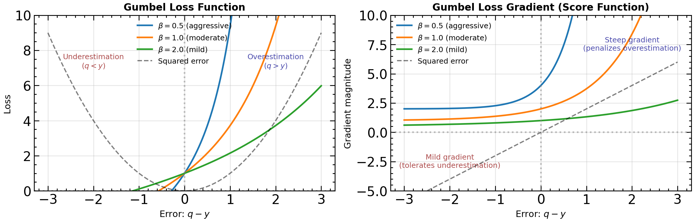

The left panel shows the Gumbel loss as a function of the error $q - y$. Notice the asymmetry: the loss grows exponentially for positive errors (overestimation) but increases only linearly for negative errors (underestimation). The parameter $\beta$ controls the degree of this asymmetry—smaller $\beta$ values create more aggressive penalization of overestimation.

The right panel shows the gradient (score function), which determines how strongly the optimizer pushes back against errors. For overestimation ($q > y$), the gradient grows exponentially, creating strong corrective pressure. For underestimation ($q < y$), the gradient remains relatively flat (approaching $1/\beta$). This is in stark contrast to squared error (dashed line), which treats over- and underestimation symmetrically. By tuning $\beta$, we can calibrate how aggressively the loss combats the overestimation bias induced by the max operator in the Bellman target.

The practical advantage of XQL is that the loss function itself handles the asymmetric error structure through its score function. We do not need to estimate variances or compute weighted averages. XQL has shown improvements in both value-based and actor-critic methods, particularly in offline reinforcement learning where the max-operator bias compounds across iterations without corrective exploration.

Classification-Based Q-Learning¶

From the buffer viewpoint, nothing changes upstream: we still sample transitions from $\hat{P}_{\mathcal{B}_t}$ and apply the same target function $g(\cdot; \boldsymbol{\theta}_t)$. Classification-based Q-learning changes only the loss $\ell$ and target representation. Instead of regressing on a scalar $y\in\mathbb{R}$ with L2, we represent values as categorical distributions over bins and use cross-entropy loss.

Choose a finite grid $z_1 < z_2 < \cdots < z_K$ spanning plausible return values. The network outputs logits $\ell_{\boldsymbol{\theta}}(s,a) \in \mathbb{R}^K$ converted to probabilities:

Each scalar TD target $y_i$ is converted to a target distribution via the two-hot encoding. If $y_i$ falls between bins $z_j$ and $z_{j+1}$:

This is barycentric interpolation: $\sum_k z_k q_k(y_i) = y_i$ recovers the scalar exactly, placing the two-hot encoding within the same framework as linear interpolation in the dynamic programming chapter (Algorithm Algorithm 2).

Source

#  label: fig-two-hot
#  caption: Two-hot encoding as barycentric interpolation: the left panel shows a single target spread over two bins, while the right panel compares encodings for multiple targets.

%config InlineBackend.figure_format = 'retina'
import numpy as np
import matplotlib.pyplot as plt

# Apply book style
try:
    import scienceplots
    plt.style.use(['science', 'notebook'])
except (ImportError, OSError):
    pass  # Use matplotlib defaults

def two_hot_encode(y, z_bins):
    """Compute two-hot encoding weights for target value y on grid z_bins."""
    K = len(z_bins)
    q = np.zeros(K)
    
    # Clip to grid boundaries
    if y <= z_bins[0]:
        q[0] = 1.0
        return q, 0
    if y >= z_bins[-1]:
        q[-1] = 1.0
        return q, K - 1
    
    # Find bins j, j+1 such that z_j <= y < z_{j+1}
    j = np.searchsorted(z_bins, y, side='right') - 1
    
    # Barycentric coordinates (linear interpolation)
    q[j+1] = (y - z_bins[j]) / (z_bins[j+1] - z_bins[j])
    q[j] = (z_bins[j+1] - y) / (z_bins[j+1] - z_bins[j])
    
    return q, j

# Set up the figure with two panels
fig, (ax1, ax2) = plt.subplots(1, 2, figsize=(12, 4))

# Define a grid of K=11 bins spanning [-5, 5]
K = 11
z_bins = np.linspace(-5, 5, K)

# Panel 1: Two-hot encoding for a specific target
y_target = 0.7
q, j = two_hot_encode(y_target, z_bins)

# Plot bins as vertical lines
for z in z_bins:
    ax1.axvline(z, color='lightgray', linestyle='--', linewidth=0.8, alpha=0.5)

# Plot the distribution
colors_bar = ['#E63946' if qi > 0 else '#A8DADC' for qi in q]
ax1.bar(z_bins, q, width=(z_bins[1] - z_bins[0]) * 0.8, 
        color=colors_bar, alpha=0.7, edgecolor='black', linewidth=1.5)

# Highlight the target value
ax1.axvline(y_target, color='#2E86AB', linewidth=3, label=f'Target $y = {y_target}$', zorder=10)
ax1.plot(y_target, 0, 'o', color='#2E86AB', markersize=12, zorder=11)

# Annotate the two active bins with barycentric coordinates
ax1.annotate(f'$q_{{{j}}} = {q[j]:.3f}$\n$= \\frac{{z_{{{j+1}}} - y}}{{z_{{{j+1}}} - z_{{{j}}}}}$',
            xy=(z_bins[j], q[j]), xytext=(z_bins[j] - 1.8, q[j] + 0.25),
            fontsize=10, color='#E63946', weight='bold',
            arrowprops=dict(arrowstyle='->', color='#E63946', lw=2))
ax1.annotate(f'$q_{{{j+1}}} = {q[j+1]:.3f}$\n$= \\frac{{y - z_{{{j}}}}}{{z_{{{j+1}}} - z_{{{j}}}}}$',
            xy=(z_bins[j+1], q[j+1]), xytext=(z_bins[j+1] + 0.5, q[j+1] + 0.25),
            fontsize=10, color='#E63946', weight='bold',
            arrowprops=dict(arrowstyle='->', color='#E63946', lw=2))

# Verify barycentric property
reconstruction = np.sum(z_bins * q)
textstr = f'Barycentric property:\n$\\sum_k z_k q_k(y) = {reconstruction:.4f} = y$'
ax1.text(0.02, 0.97, textstr, transform=ax1.transAxes, fontsize=10,
        verticalalignment='top', bbox=dict(boxstyle='round', facecolor='wheat', alpha=0.8))

ax1.set_xlabel('Bin value $z_k$', fontsize=11)
ax1.set_ylabel('Probability $q_k(y)$', fontsize=11)
ax1.set_title('Two-Hot Encoding = Linear Interpolation', fontsize=12, fontweight='bold')
ax1.set_ylim([0, 1.2])
ax1.legend(loc='upper right', fontsize=10)
ax1.grid(axis='y', alpha=0.3)

# Panel 2: Multiple targets to show the pattern
targets = [0.7, -2.3, 3.8]
colors = ['#2E86AB', '#A23B72', '#F18F01']

for idx, (y_target, color) in enumerate(zip(targets, colors)):
    q, _ = two_hot_encode(y_target, z_bins)
    offset = idx * 0.2
    ax2.bar(z_bins + offset, q, width=0.18, color=color, alpha=0.7, 
           label=f'$y = {y_target}$', edgecolor='black', linewidth=0.8)

for z in z_bins:
    ax2.axvline(z, color='lightgray', linestyle='--', linewidth=0.5, alpha=0.4)

ax2.set_xlabel('Bin value $z_k$', fontsize=11)
ax2.set_ylabel('Probability $q_k(y)$', fontsize=11)
ax2.set_title('Multiple Targets: Each Encoded as Two-Hot', fontsize=12, fontweight='bold')
ax2.legend(loc='upper right', fontsize=10)
ax2.grid(axis='y', alpha=0.3)

plt.tight_layout()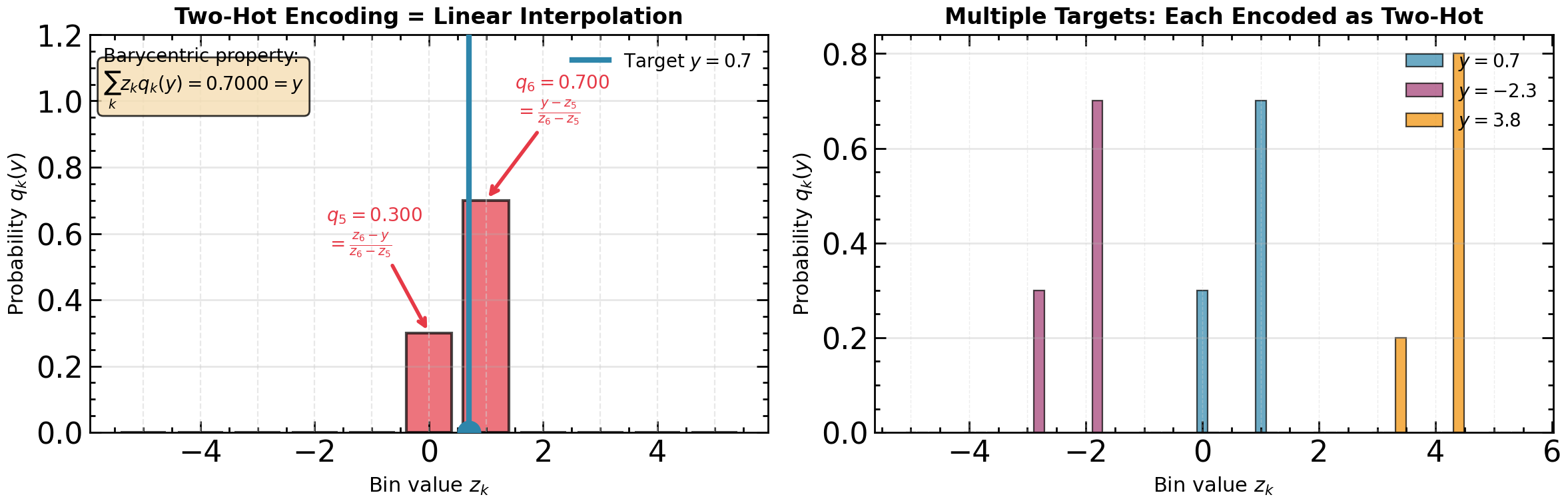

The left panel shows two-hot encoding for $y=0.7$ on a grid of 11 bins. The target value is distributed over exactly two adjacent bins $z_j$ and $z_{j+1}$ with weights that are barycentric coordinates: the weight assigned to each bin is inversely proportional to the distance from the target to that bin. The inset verifies that $\sum_k z_k q_k(y)$ exactly recovers the original target—this is the same linear interpolation formula used throughout the book. The right panel shows that different targets produce different two-hot patterns, each concentrating mass on the two bins surrounding the target value.

The loss minimizes cross-entropy:

which projects the target distribution onto the predicted distribution in KL geometry on the simplex $\Delta^{K-1}$ rather than L2 on $\mathbb{R}$. The gradient is $\nabla_{\ell_\theta} \mathcal{L}_{\text{CE}} = p_\theta - q$, bounded in magnitude regardless of target size.

This provides three sources of implicit robustness. First, gradient influence is bounded: each sample contributes $O(1)$ gradient magnitude per bin, unlike L2 where error magnitude $E$ contributes gradient proportional to $E$. Second, the finite grid $[z_1, z_K]$ clips extreme targets to boundary bins, preventing outliers from dominating the regression scale. Third, the two-hot encoding spreads mass across neighboring bins, providing label smoothing that averages noisy targets at the same $(s,a)$.

The two-hot weights $q_j(y_i), q_{j+1}(y_i)$ are barycentric coordinates, identical to linear interpolation in the dynamic programming chapter (Algorithm Algorithm 2). This places the encoding within Gordon’s monotone approximator framework (Definition Definition 1): targets are convex combinations preserving order and boundedness. The neural network predicting $p_{\boldsymbol{\theta}}(\cdot \mid s,a)$ is non-monotone, making classification-based Q-learning a hybrid: monotone target structure paired with flexible function approximation.

Empirically, cross-entropy loss scales better with network capacity. Farebrother et al. Farebrother et al. (2024) found that L2-based DQN and CQL degrade when Q-networks scale to large ResNets, while classification loss (specifically HL-Gauss, which uses Gaussian smoothing instead of two-hot) maintains performance. The combination of KL geometry, quantization, and smoothing prevents overfitting to noisy targets that plagues L2 with high-capacity networks.

Summary¶

Fitted Q-iteration has a two-level structure: an outer loop applies the Bellman operator to construct targets, an inner loop fits a function approximator to those targets. All algorithms in this chapter instantiate this template with different choices of buffer $\mathcal{B}_t$, target function $g$, loss $\ell$, and optimization budget $K$.

The empirical distribution $\hat{P}_{\mathcal{B}_t}$ unifies offline and online methods through plug-in approximation: replace unknown transition law $P$ with $\hat{P}_{\mathcal{B}_t}$ and minimize empirical risk $\mathbb{E}_{((s,a),y)\sim \hat{P}_t^{\text{fit}}} [\ell(q, y)]$. Offline uses fixed $\mathcal{B}_t \equiv \mathcal{D}$ (sample average approximation), online uses circular buffer (Q-learning with $B=1$ is stochastic approximation, DQN with large $B$ is hybrid).

Target networks and online networks arise from flattening the nested loops. Merging inner gradient steps with outer value iteration creates a single loop where two sets of parameters coexist: the online network $\boldsymbol{\theta}_t$ (actively updated at each gradient step, corresponds to $\boldsymbol{\theta}_n^{(k)}$) and the target network $\boldsymbol{\theta}_{\text{target}}$ (frozen for computing targets, updated every $K$ steps to mark outer-iteration boundaries, corresponds to $\boldsymbol{\theta}_n$). In online algorithms like DQN, the online network additionally serves as the behavior policy for data collection.

The next chapter directly parameterizes and optimizes policies instead of searching over value functions.