Discrete-Time Trajectory Optimization

In the previous chapter, we examined different ways to represent dynamical systems: continuous versus discrete time, deterministic versus stochastic, fully versus partially observable, and even simulation-based views such as agent-based or programmatic models. Our focus was on the structure of models: how they capture evolution, uncertainty, and information.

In this chapter, we turn to what makes these models useful for decision-making. The goal is no longer just to describe how a system behaves, but to leverage that description to compute actions over time. This doesn’t mean the model prescribes actions on its own. Rather, it provides the scaffolding for optimization: given a model and an objective, we can derive the control inputs that make the modeled system behave well according to a chosen criterion.

Our entry point will be trajectory optimization. By a trajectory, we mean the time-indexed sequence of states and controls that the system follows under a plan: the states $(\mathbf{x}_1, \dots, \mathbf{x}_T)$ together with the controls $(\mathbf{u}_1, \dots, \mathbf{u}_{T-1})$. In this chapter, we focus on an open-loop viewpoint: starting from a known initial state, we compute the entire sequence of controls in advance and then apply it as-is. This is appealing because, for discrete-time problems, it yields a finite-dimensional optimization over a vector of decisions and cleanly exposes the structure of the constraints. In continuous time, the base formulation is infinite-dimensional; in this course we will rely on direct methods (time discretization and parameterization) to transform it into a finite-dimensional nonlinear program.

Open loop also has a clear limitation: if reality deviates from the model, whether due to disturbances, model mismatch, or unanticipated events, the state you actually reach may differ from the predicted one. The precomputed controls that were optimal for the nominal trajectory can then lead you further off course, and errors can compound over time.

Later, we will study closed-loop (feedback) strategies, where the choice of action at time $t$ can depend on the state observed at time $t$. Instead of a single sequence, we optimize a policy $\pi_t$ mapping states to controls, $\mathbf{u}_t = \pi_t(\mathbf{x}_t)$. Feedback makes plans resilient to unforeseen situations by adapting on the fly, but it leads to a more challenging problem class. We start with open-loop trajectory optimization to build core concepts and tools before tackling feedback design.

A Motivating Example: Inventory Control¶

Before diving into the general formulation, consider a concrete problem that arises in operations management. A retailer must decide how much inventory to order at the start of each period to meet uncertain demand while balancing holding costs against stockout penalties.

The setup is simple. At the beginning of period $k$, the retailer observes the current inventory level $x_k$ and places an order of size $u_k \ge 0$. Demand $d_k$ then arrives (assume for now it is known in advance), and the inventory evolves according to

If inventory is positive at the end of the period, holding costs accrue. If inventory is negative (backorders), penalty costs apply. There may also be a per-unit ordering cost. A typical objective is to minimize total cost over a planning horizon of $T$ periods:

where $[z]_+ = \max(0,z)$, $h$ is the holding cost rate, $p$ is the backorder penalty rate, and $c$ is the ordering cost per unit. The retailer may also face constraints: orders cannot be negative, and inventory might be bounded above by warehouse capacity.

This problem has a clear structure: a state ($x_k$) that evolves according to a known rule, a control ($u_k$) that influences the next state, a cost that accumulates over time, and constraints on the decisions. These ingredients define a discrete-time optimal control problem (DOCP). We now formalize this structure in general terms.

Discrete-Time Optimal Control Problems (DOCPs)¶

Consider a system described by a state $\mathbf{x}_t \in \mathbb{R}^n$, summarizing everything needed to predict its evolution. At each stage $t$, we can influence the system through a control input $\mathbf{u}_t \in \mathbb{R}^m$. The dynamics specify how the state evolves:

where $\mathbf{f}_t$ may be nonlinear or time-varying. We assume the initial state $\mathbf{x}_1$ is known.

The goal is to pick a sequence of controls $\mathbf{u}_1,\dots,\mathbf{u}_{T-1}$ that makes the trajectory desirable. But desirable in what sense? That depends on an objective function, which often includes two components:

The stage cost reflects ongoing penalties such as energy, delay, or risk. The terminal cost measures the value (or cost) of ending in a particular state. Together, these give a discrete-time Bolza problem with path constraints and bounds:

Returning to the inventory example, the correspondence is direct: the state $\mathbf{x}_t$ is the inventory level $x_k$, the control $\mathbf{u}_t$ is the order quantity $u_k$, and the dynamics $\mathbf{f}_t$ encode the inventory balance equation $x_{k+1} = x_k + u_k - d_k$. The stage cost $c_t$ captures holding, backorder, and ordering costs, while the terminal cost $c_T$ might penalize ending with excess stock. Constraints $\mathbf{g}_t \le \mathbf{0}$ can enforce non-negativity of orders or warehouse capacity limits. This mapping shows how practical problems fit naturally into the abstract framework.

Written this way, it may seem obvious that the decision variables are the controls $\mathbf{u}_t$. After all, in most intuitive descriptions of control, we think of choosing inputs to influence the system. But notice that in the program above, the entire state trajectory also appears as a set of variables, linked to the controls by the dynamics constraints. This is intentional: it reflects one way of writing the problem that makes the constraints explicit.

Why introduce $\mathbf{x}_t$ as decision variables if they can be simulated forward from the controls? Many readers hesitate here, and the question is natural: If the model is deterministic and $\mathbf{x}_1$ is known, why not pick $\mathbf{u}_{1:T-1}$ and compute $\mathbf{x}_{2:T}$ on the fly? That instinct leads to single shooting, a method we will return to shortly.

Already in this formulation, though, the structure of the problem matters. Ignoring it can make our life much harder. The reason is twofold:

• Dimensionality grows with the horizon. For a horizon of length $T$, the program has roughly $(T-1)(m+n)$ decision variables.

• Temporal coupling. Each control affects all future states and costs. The feasible set is not a simple box but a narrow manifold defined by the dynamics.

Together, these features explain why specialized methods exist and why the way we write the problem influences the algorithms we can use. Whether we keep states explicit or eliminate them through forward simulation determines not just the problem size, but also its conditioning and the trade-offs between robustness and computational effort.

Existence of Solutions and Optimality Conditions¶

Now that we have the optimization problem written down, we can ask: does it always have a solution? And if so, how do we recognize one? These questions lead us to feasibility and optimality conditions.

Existence of Solutions¶

Notice first that nothing in the problem statement required the dynamics

to be stable. In fact, many problems of interest involve unstable systems; think of balancing a pole or steering a spacecraft. What matters is that the dynamics are well defined: given a state–control pair, the rule $\mathbf{f}_t$ produces a valid next state.

In continuous time, one usually requires $\mathbf{f}$ to be continuous (often Lipschitz continuous) in $\mathbf{x}$ so that the ODE has a unique solution on the horizon of interest. In discrete time, the requirement is lighter: we only need the update map to be well posed.

Existence also hinges on feasibility. A candidate control sequence must generate a trajectory that respects all constraints: the dynamics, any bounds on state and control, and any terminal requirements. If no such sequence exists, the feasible set is empty and the problem has no solution. This can happen if the constraints are overly strict, or if the system is uncontrollable from the given initial condition.

Optimality Conditions¶

Assume the feasible set is nonempty. To characterize a point that is not only feasible but locally optimal, we use the Lagrange multiplier machinery from nonlinear programming. For a smooth problem

define the Lagrangian

For an inequality system $H(\mathbf{z})\ge \mathbf{0}$ and a candidate point $\mathbf{z}$, the active set is

while indices with $H_i(\mathbf{z})>0$ are inactive. Only active inequalities can carry positive multipliers.

We now make a constraint qualification assumption. In plain language, it says the constraints near the solution intersect in a regular way so that the feasible set has a well-defined tangent space and the multipliers exist. Algebraically, this amounts to a full row rank condition on the Jacobian of the equalities together with the active inequalities:

This is the LICQ (Linear Independence Constraint Qualification). In convex problems, Slater’s condition (existence of a strictly feasible point) plays a similar role. You can think of these as the assumptions that let the linearized KKT equations be solvable; we do not literally invert that Jacobian, but the full-rank property is what would make such an inversion possible in principle.

Under such a constraint qualification, any local minimizer $\mathbf{z}^\star$ admits multipliers $(\boldsymbol{\lambda}^\star,\boldsymbol{\mu}^\star)$ that satisfy the Karush–Kuhn–Tucker (KKT) conditions:

Only constraints that are active at $\mathbf{z}^\star$ can have $\mu_i^\star>0$; inactive ones have $\mu_i^\star=0$. The multipliers quantify marginal costs: $\lambda_j^\star$ measures how the optimal value changes if the $j$-th equality is relaxed, and $\mu_i^\star$ does the same for the $i$-th inequality. (If you prefer $h(\mathbf{z})\le 0$, signs flip accordingly.)

In our trajectory problems, $\mathbf{z}$ stacks state and control trajectories, $G$ enforces the dynamics, and $H$ collects bounds and path constraints. The equalities’ multipliers act as costates or shadow prices for the dynamics. Writing the KKT system stage by stage yields the discrete-time Pontryagin principle, derived next. For convex programs these conditions are also sufficient.

What fails without a CQ? If the active gradients are dependent (for example duplicated or nearly parallel), the Jacobian loses rank; multipliers may then be nonunique or fail to exist, and the linearized equations become ill-posed. In transcribed trajectory problems this shows up as dependent dynamic constraints or redundant path constraints, which leads to fragile solver behavior.

Recap. The KKT conditions provide necessary conditions for a point to be a local minimizer of a constrained optimization problem. They consist of four parts: stationarity (the gradient of the Lagrangian vanishes), primal feasibility (constraints are satisfied), dual feasibility (inequality multipliers are nonnegative), and complementarity (inactive constraints have zero multipliers). The multipliers have an economic interpretation as marginal costs—they tell us how much the optimal value would change if we relaxed a constraint slightly. For convex problems, the KKT conditions are also sufficient, meaning any point satisfying them is globally optimal. In trajectory optimization, these conditions will reappear in structured form as the Pontryagin principle.

From KKT to algorithms¶

The KKT system can be read as the first-order optimality conditions of a saddle-point problem. With equalities $G(\mathbf{z})=\mathbf{0}$ and inequalities $H(\mathbf{z})\ge \mathbf{0}$, define the Lagrangian

Optimality corresponds to a saddle: minimize in $\mathbf{z}$, maximize in $(\boldsymbol{\lambda},\boldsymbol{\mu})$ (with $\boldsymbol{\mu}$ constrained to the nonnegative orthant).

Primal–dual gradient dynamics (Arrow–Hurwicz)¶

The simplest algorithm mirrors this saddle structure by descending in the primal variables and ascending in the dual variables, with a projection for the inequalities:

Here $\Pi_{\ge 0}$ is the projection onto $\{\boldsymbol{\mu}\ge 0\}$. In convex settings and with suitable step sizes, these iterates converge to a saddle point. In nonconvex problems (our trajectory optimizations after transcription), these updates are often used inside augmented Lagrangian or penalty frameworks to improve robustness, for example by replacing $\mathcal{L}$ with

which stabilizes the dual ascent when constraints are not yet well satisfied.

SQP as Newton on the KKT system (equality case)¶

With only equality constraints $G(\mathbf{z})=\mathbf{0}$, write first-order conditions

Applying Newton’s method to this system gives the linear KKT solve

This is exactly the step computed by Sequential Quadratic Programming (SQP) in the equality-constrained case: it is Newton’s method on the KKT equations. For general problems with inequalities, SQP forms a quadratic subproblem by quadratically modeling $F$ with $\nabla_{\mathbf{z}\mathbf{z}}^2\mathcal{L}$ and linearizing the constraints, then solves that QP with line search or trust region. In least-squares-like problems one often uses Gauss–Newton (or a Levenberg–Marquardt trust region) as a positive-definite approximation to the Lagrangian Hessian.

In trajectory optimization, the KKT matrix inherits banded/sparse structure from the dynamics. Newton/SQP steps can be computed efficiently by exploiting this structure; in the special case of quadratic models and linearized dynamics, the QP reduces to an LQR solve along the horizon (this is the backbone of iLQR/DDP-style methods). Primal-dual updates provide simpler iterations and are easy to implement; augmented terms are typically needed to obtain stable progress when constraints couple stages.

The choice between methods depends on the context. Primal-dual gradients give lightweight iterations and are suited for warm starts or as inner loops with penalties. SQP/Newton gives rapid local convergence when close to a solution and LICQ holds; trust regions or line search help globalize convergence.

Examples of DOCPs¶

To make things concrete, here are additional problems that are naturally posed as discrete-time OCPs. We already introduced inventory control at the start of this chapter; below are two more examples from different domains, followed by a discussion of how continuous-time problems give rise to DOCPs through discretization.

End-of-Day Portfolio Rebalancing¶

At each trading day $k$, choose trades $u_k$ to adjust holdings $h_k$ before next-day returns $r_{k}$ realize. Deterministic planning uses predicted returns $\mu_k$, with dynamics $h_{k+1} = (h_k + u_k) \odot (\mathbf{1} + \mu_k)$ and budget/box constraints. The stage cost can capture transaction costs and risk, e.g., $c_k(h_k,u_k) = \tau\lVert u_k \rVert_1 + \tfrac{\lambda}{2}\,h_k^\top \Sigma_k h_k$, with a terminal utility or wealth objective.

Daily Ad-Budget Allocation with Carryover¶

Allocate spend $u_k \in [0, U_{\max}]$ to build awareness $s_k$ with carryover dynamics $s_{k+1} = \alpha s_k + \beta u_k$. Conversions/revenue at day $k$ follow a response curve $g(s_k,u_k)$; the goal is $\max \sum_{k=0}^{T-1} g(s_k,u_k) - c\,u_k$ subject to spend limits. This is naturally discrete because decisions and measurements occur daily.

DOCPs Arising from the Discretization of Continuous-Time OCPs¶

Although many applications are natively discrete-time, it is also common to obtain a DOCP by discretizing a continuous-time formulation. Consider a system on $[0, T_c]$ given by

Choose a step size $\Delta > 0$ and grid $t_k = k\,\Delta$. A one-step integration scheme induces a discrete map $\mathbf{F}_\Delta$ so that

where, for example, explicit Euler gives $\mathbf{F}_\Delta(\mathbf{x},\mathbf{u},t) = \mathbf{x} + \Delta\,\mathbf{f}(t,\mathbf{x},\mathbf{u})$. The resulting discrete-time optimal control problem takes the Bolza form with these induced dynamics:

Programs as DOCPs and Differentiable Programming¶

It is often useful to view a computer program itself as a discrete-time dynamical system. Let the program state collect memory, buffers, and intermediate variables, and let the control represent inputs or tunable decisions at each step. A single execution step defines a transition map

and a scalar objective (e.g., loss, error, runtime, energy) yields a DOCP:

In differentiable programming (e.g., JAX, PyTorch), the composed map $\Phi_{T-1}\circ\cdots\circ\Phi_0$ is differentiable, enabling reverse-mode automatic differentiation and efficient gradient-based trajectory optimization. When parts of the program are non-differentiable (discrete branches, simulators with events), DOCPs can still be solved using derivative-free or weak-gradient methods (eg. finite differences, SPSA, Nelder–Mead, CMA-ES, or evolutionary strategies) optionally combined with smoothing, relaxations, or stochastic estimators to navigate non-smooth regions.

Example: Retry Loop Optimization¶

Consider a simple retry loop that attempts an operation up to $K$ times, waiting $u_k$ seconds before the $k$-th attempt. The server has time-varying availability: it is unreliable early on but recovers after a transient outage. The goal is to find a wait schedule that minimizes expected latency while ensuring eventual success.

We cast this as a DOCP. The state $x_k = (t, k, \text{done})$ tracks elapsed time, attempt count, and success status. The control $u_k \in [0, 2]$ is the wait before attempt $k$. The transition applies the wait, then flips a biased coin based on current server availability. The cost penalizes total time and failure.

Source

#  label: fig-ocp-retry-loop
#  caption: SPSA optimization of a retry schedule. The optimized schedule waits longer initially, allowing the server to recover before retrying.

%config InlineBackend.figure_format = 'retina'
import random
import matplotlib.pyplot as plt

try:
    import scienceplots
    plt.style.use(['science', 'notebook'])
except (ImportError, OSError):
    pass

# Server availability: low initially, recovers after t=1.5s
def success_prob(t):
    return 0.2 if t < 1.5 else 0.85

# One step of the retry program
def step(state, u_k):
    t, k, done = state
    if done:
        return (t, k, True)
    t_new = t + max(0.0, min(2.0, u_k))  # apply wait (clipped)
    success = random.random() < success_prob(t_new)
    return (t_new, k + 1, success)

# Rollout: run the retry loop, return total cost
def rollout(u, seed=0):
    random.seed(seed)
    state = (0.0, 0, False)  # (time, attempts, done)
    for k in range(len(u)):
        state = step(state, u[k])
        if state[2]:  # success
            break
    t, attempts, done = state
    return t + (5.0 if not done else 0.0)  # penalize failure

# SPSA optimization
def spsa_optimize(K=6, iters=150, seed=0):
    random.seed(seed)
    u = [0.2] * K  # initial schedule: short waits
    alpha, c0 = 0.15, 0.1
    for i in range(1, iters + 1):
        c = c0 / (i ** 0.1)
        delta = [1 if random.random() < 0.5 else -1 for _ in range(K)]
        u_plus = [max(0, min(2, u[j] + c * delta[j])) for j in range(K)]
        u_minus = [max(0, min(2, u[j] - c * delta[j])) for j in range(K)]
        Jp = sum(rollout(u_plus, seed=seed + 2*i) for _ in range(8)) / 8
        Jm = sum(rollout(u_minus, seed=seed + 2*i + 1) for _ in range(8)) / 8
        g = [(Jp - Jm) / (2 * c * delta[j]) for j in range(K)]
        u = [max(0, min(2, u[j] - alpha * g[j])) for j in range(K)]
    return u

K = 6
u_init = [0.2] * K
u_opt = spsa_optimize(K=K, iters=150, seed=42)

# Evaluate costs (average over seeds)
cost_init = sum(rollout(u_init, seed=s) for s in range(50)) / 50
cost_opt = sum(rollout(u_opt, seed=s) for s in range(50)) / 50

print(f"Initial schedule: {[round(x, 2) for x in u_init]}  Avg cost: {cost_init:.2f}")
print(f"Optimized schedule: {[round(x, 2) for x in u_opt]}  Avg cost: {cost_opt:.2f}")

fig, ax = plt.subplots(figsize=(7, 4))
attempts = range(1, K + 1)
ax.step(attempts, u_init, where="mid", label=f"Initial (cost={cost_init:.2f})", linestyle="--")
ax.step(attempts, u_opt, where="mid", label=f"Optimized (cost={cost_opt:.2f})")
ax.set_xlabel("Attempt")
ax.set_ylabel("Wait time (s)")
ax.set_title("Retry Schedule Optimization via SPSA")
ax.legend()
ax.grid(alpha=0.3)
fig.tight_layout()

Initial schedule: [0.2, 0.2, 0.2, 0.2, 0.2, 0.2]  Avg cost: 2.35
Optimized schedule: [0.26, 0.15, 0.34, 0.85, 0.15, 0.77]  Avg cost: 1.07

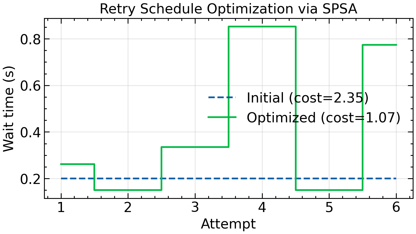
The optimized schedule learns to wait longer before early attempts, giving the server time to recover from the outage. This simple example illustrates how viewing a program as a dynamical system enables trajectory optimization even when the transition involves stochastic branching.

Example: Gradient Descent with Momentum as DOCP¶

To connect this lens to familiar practice, including hyperparameter optimization, treat the learning rate and momentum (or their schedules) as controls. Rather than fixing them a priori, we can optimize them as part of a trajectory optimization. The optimizer itself becomes the dynamical system whose execution we shape to minimize final loss.

Program: gradient descent with momentum on a quadratic loss. We fit $\boldsymbol{\theta}\in\mathbb{R}^p$ to data $(\mathbf{A},\mathbf{b})$ by minimizing

The program maintains parameters $\boldsymbol{\theta}_k$ and momentum $\mathbf{m}_k$. Each iteration does:

1. compute gradient $\mathbf{g}_k=\nabla_{\boldsymbol{\theta}}\ell(\boldsymbol{\theta}_k)=\mathbf{A}^\top(\mathbf{A}\boldsymbol{\theta}_k-\mathbf{b})$

2. update momentum $\mathbf{m}_{k+1}=\beta_k \, \mathbf{m}_k + \mathbf{g}_k$

3. update parameters $\boldsymbol{\theta}_{k+1}=\boldsymbol{\theta}_k - \alpha_k \, \mathbf{m}_{k+1}$

State, control, and transition. Define the state $\mathbf{x}_k=\begin{bmatrix}\boldsymbol{\theta}_k\\ \mathbf{m}_k\end{bmatrix}\in\mathbb{R}^{2p}$ and the control $\mathbf{u}_k=\begin{bmatrix}\alpha_k\\ \beta_k\end{bmatrix}$. One program step is

Executing the program for $T$ iterations gives the trajectory

Objective as a DOCP. Choose terminal cost $c_T(\mathbf{x}_T)=\ell(\boldsymbol{\theta}_T)$ and (optionally) stage costs $c_k(\mathbf{x}_k,\mathbf{u}_k)=\rho_\alpha \, \alpha_k^2+\rho_\beta\,(\beta_k- \bar\beta)^2$. The program-as-control problem is

Backpropagation = reverse-time costate recursion. Because $\Phi_k$ is differentiable, reverse-mode AD computes $\nabla_{\mathbf{u}_{0:T-1}} \big(c_T+\sum c_k\big)$ by propagating a costate $\boldsymbol{\lambda}_k=\partial \mathcal{J}/\partial \mathbf{x}_k$ backward:

and the gradients with respect to controls are

Unrolling a tiny horizon ($T=3$) to see the composition:

What if the program branches? Suppose we insert a “skip-small-gradients” branch

which is non-differentiable because of the indicator. The DOCP view still applies, but gradients are unreliable. Two practical paths: smooth the branch (e.g., replace $\mathbf{1}\{\cdot\}$ with $\sigma((\lVert\mathbf{g}_k\rVert-\tau)/\epsilon)$ for small $\epsilon$) and use autodiff; or go derivative-free on $\{\alpha_k,\beta_k,\tau\}$ (e.g., SPSA or CMA-ES) while keeping the inner dynamics exact.

Variants: Lagrange and Mayer Problems¶

The Bolza form is general enough to cover most situations, but two common special cases deserve mention:

• Lagrange problem (no terminal cost) If the objective only accumulates stage costs:

Example: Energy minimization for a delivery drone. The concern is total battery use, regardless of the final position.

• Mayer problem (terminal cost only) If the objective depends only on the final state:

Example: Satellite orbital transfer. The only goal is to reach a specified orbit, no matter the fuel spent along the way.

These distinctions matter when deriving optimality conditions, but conceptually they fit in the same framework: the system evolves over time, and we choose controls to shape the trajectory.

Reducing to Mayer Form by State Augmentation¶

Although Bolza, Lagrange, and Mayer problems look different, they are equivalent in expressive power. Any problem with running costs can be rewritten as a Mayer problem (one whose objective depends only on the final state) through a simple trick: augment the state with a running sum of costs.

The idea is straightforward. Introduce a new variable, $y_t$, that keeps track of the cumulative cost so far. At each step, we update this running sum along with the system state:

where $\tilde{\mathbf{x}}_t = (\mathbf{x}_t, y_t)$. The terminal cost then becomes:

The overall effect is that the explicit sum $\sum_{t=1}^{T-1} c_t(\mathbf{x}_t,\mathbf{u}_t)$ disappears from the objective and is captured implicitly by the augmented state. This lets us write every optimal control problem in Mayer form.

This reduction serves two purposes. First, it often simplifies mathematical derivations, as we will see later when deriving necessary conditions. Second, it can streamline algorithmic implementation: instead of writing separate code paths for Mayer, Lagrange, and Bolza problems, we can reduce everything to one canonical form. That said, this unified approach is not always best in practice. Specialized formulations can sometimes be more efficient computationally, especially when the running cost has simple structure.

The unifying theme is that a DOCP may look like a generic NLP on paper, but its structure matters. Ignoring that structure often leads to impractical solutions, whereas formulations that expose sparsity and respect temporal coupling allow modern solvers to scale effectively. In the following sections, we will examine how these choices play out in practice through single shooting, multiple shooting, and collocation methods, and why different formulations strike different trade-offs between robustness and computational effort.

Numerical Methods for Solving DOCPs¶

Before we discuss specific algorithms, it is useful to clarify the goal: we want to recast a discrete-time optimal control problem as a standard nonlinear program (NLP). Collect all decision variables (states, controls, and any auxiliary variables) into a single vector $\mathbf{z}\in\mathbb{R}^{n_z}$ and write

with maps $F:\mathbb{R}^{n_z}\to\mathbb{R}$, $G:\mathbb{R}^{n_z}\to\mathbb{R}^{r_e}$, and $H:\mathbb{R}^{n_z}\to\mathbb{R}^{r_h}$. In optimal control, $G$ typically encodes dynamics and boundary conditions, while $H$ captures path and box constraints.

There are multiple ways to arrive at (and benefit from) this NLP:

• Simultaneous (direct transcription / full discretization): keep all states and controls as variables and impose the dynamics as equality constraints. This is straightforward and exposes sparsity, but the problem can be large unless solver-side techniques (e.g., condensing) are exploited.

• Sequential (recursive elimination / single shooting): eliminate states by forward propagation from the initial condition, leaving controls as the main decision variables. This reduces dimension and constraints, but can be sensitive to initialization and longer horizons.

• Multiple shooting: introduce state variables at segment boundaries and enforce continuity between simulated segments. This compromises between size and conditioning and is often more robust than pure single shooting.

The next sections work through these formulations, starting with simultaneous methods, then sequential methods, and finally multiple shooting, before discussing how generic NLP solvers and specialized algorithms leverage the resulting structure in practice.

Simultaneous Methods¶

In the simultaneous (also called direct transcription or full discretization) approach, we keep the entire trajectory explicit and enforce the dynamics as equality constraints. Starting from the Bolza DOCP,

collect all variables into a single vector

Path constraints typically apply only at selected times. Let $\mathscr{E}$ index additional equality constraints $g_i$ and $\mathscr{I}$ index inequality constraints $h_i$. For each constraint $i$, define the set of time indices $K_i \subseteq \{1,\dots,T\}$ where it is enforced (e.g., terminal constraints use $K_i = \{T\}$). The simultaneous transcription is the NLP

optionally with simple bounds $\mathbf{x}_{\mathrm{lb}} \le \mathbf{x}_t \le \mathbf{x}_{\mathrm{ub}}$ and $\mathbf{u}_{\mathrm{lb}} \le \mathbf{u}_t \le \mathbf{u}_{\mathrm{ub}}$ folded into $H$ or provided to the solver separately. For notational convenience, some constraints may not depend on $\mathbf{u}_k$ at times in $K_i$; the indexing still helps specify when each condition is active.

This direct transcription is attractive because it is faithful to the model and exposes sparsity. The Jacobian of $G$ has a block bi-diagonal structure induced by the dynamics, and the KKT matrix is sparse and structured. These properties are exploited by interior-point and SQP methods. The trade-off is size: with state dimension $n$ and control dimension $m$, the decision vector has $(T\!\cdot\!n) + ((T\!- 1)\cdot m)$ entries, and there are roughly $(T\!- 1)\cdot n$ dynamic equalities plus any path and boundary conditions. Techniques such as partial or full condensing eliminate state variables to reduce the equality set (at the cost of denser matrices), while keeping states explicit preserves sparsity and often improves robustness on long horizons and in the presence of state constraints.

Compared to alternatives, simultaneous methods avoid the long nonlinear dependency chains of single shooting and make it easier to impose state/path constraints. They can, however, demand more memory and per-iteration linear algebra, so practical performance hinges on exploiting sparsity and good initialization.

The same logic applies when selecting an optimizer. For small-scale problems, it is common to rely on general-purpose routines such as those in scipy.optimize.minimize. Derivative-free methods like Nelder–Mead require no gradients but scale poorly as dimensionality increases. Quasi-Newton schemes such as BFGS work well for moderate dimensions and can approximate gradients by finite differences, while large-scale trajectory optimization often calls for gradient-based constrained solvers such as interior-point or sequential quadratic programming methods that can exploit sparse Jacobians and benefit from automatic differentiation. Stochastic techniques, including genetic algorithms, simulated annealing, or particle swarm optimization, occasionally appear when gradients are unavailable, but their cost grows rapidly with dimension and they are rarely competitive for structured optimal control problems.

Sequential Methods¶

The previous section showed how a discrete-time optimal control problem can be solved by treating all states and controls as decision variables and enforcing the dynamics as equality constraints. This produces a nonlinear program that can be passed to solvers such as scipy.optimize.minimize with the SLSQP method. For short horizons, this approach is straightforward and works well; the code stays close to the mathematical formulation.

It also has a real advantage: by keeping the states explicit and imposing the dynamics through constraints, we anchor the trajectory at multiple points. This extra structure helps stabilize the optimization, especially for long horizons where small deviations in early steps can otherwise propagate and cause the optimizer to drift or diverge. In that sense, this formulation is better conditioned and more robust than approaches that treat the dynamics implicitly.

The drawback is scale. As the horizon grows, the number of variables and constraints grows with it, and all are coupled by the dynamics. Each iteration of a sequential quadratic programming (SQP) or interior-point method requires building and factorizing large Jacobians and Hessians. These methods have been embedded in reinforcement learning and differentiable programming pipelines, through implicit layers or differentiable convex solvers, but the cost is significant. They remain serial, rely on repeated linear algebra factorizations, and are difficult to parallelize efficiently. When thousands of such problems must be solved inside a learning loop, the overhead becomes prohibitive.

This motivates an alternative that aligns better with the computational model of machine learning. If the dynamics are deterministic and state constraints are absent (or reducible to simple bounds on controls), we can eliminate the equality constraints altogether by making the states implicit. Instead of solving for both states and controls, we fix the initial state and roll the system forward under a candidate control sequence. This is the essence of single shooting.

The term “shooting” comes from the idea of aiming and firing a trajectory from the initial state: you pick a control sequence, integrate (or step) the system forward, and see where it lands. If the final state misses the target, you adjust the controls and try again: like adjusting the angle of a shot until it hits the mark. It is called single shooting because we compute the entire trajectory in one pass from the starting point, without breaking it into segments. Later, we will contrast this with multiple shooting, where the horizon is divided into smaller arcs that are optimized jointly to improve stability and conditioning.

The analogy with deep learning is also immediate: the control sequence plays the role of parameters, the rollout is a forward pass, and the cost is a scalar loss. Gradients can be obtained with reverse-mode automatic differentiation. In the single shooting formulation of the DOCP, the constrained program

collapses to

Here $\boldsymbol{\phi}_t$ denotes the state reached at time $t$ by recursively applying the dynamics to the previous state and current control. This recursion can be written as

Concretely, here is JAX-style pseudocode for defining phi(u, x_0, t) using jax.lax.scan with a zero-based time index:

def phi(u_seq, x0, t):
    """Return \phi_t(u, x0) with 0-based t (\phi_0 = x0).

    u_seq: controls of length T (or T-1); only first t entries are used
    x0: initial state at time 0
    t: integer >= 0
    """
    if t <= 0:
        return x0

    def step(carry, u):
        x, t_idx = carry
        x_next = f(x, u, t_idx)
        return (x_next, t_idx + 1), None

    (x_t, _), _ = lax.scan(step, (x0, 0), u_seq[:t])
    return x_t

The pattern mirrors an RNN unroll: starting from an initial state ($\mathbf{x}^\star_1$) and a sequence of controls ($\mathbf{u}^*_{1:T-1}$), we propagate forward through the dynamics, updating the state at each step and accumulating cost along the way. This structural similarity is why single shooting often feels natural to practitioners with a deep learning background: the rollout is a forward pass, and gradients propagate backward through time exactly as in backpropagation through an RNN.

Algorithmically:

In JAX or PyTorch, this loop can be JIT-compiled and differentiated automatically. Any gradient-based optimizer (L-BFGS, Adam, even SGD) can be applied, making the pipeline look very much like training a neural network. In effect, we are “backpropagating through the world model” when computing $\nabla J(\mathbf{u})$.

Single shooting is attractive for its simplicity and compatibility with differentiable programming, but it has limitations. The absence of intermediate constraints makes it sensitive to initialization and prone to numerical instability over long horizons. When state constraints or robustness matter, formulations that keep states explicit, such as multiple shooting or collocation, become preferable. These trade-offs are the focus of the next section.

Source

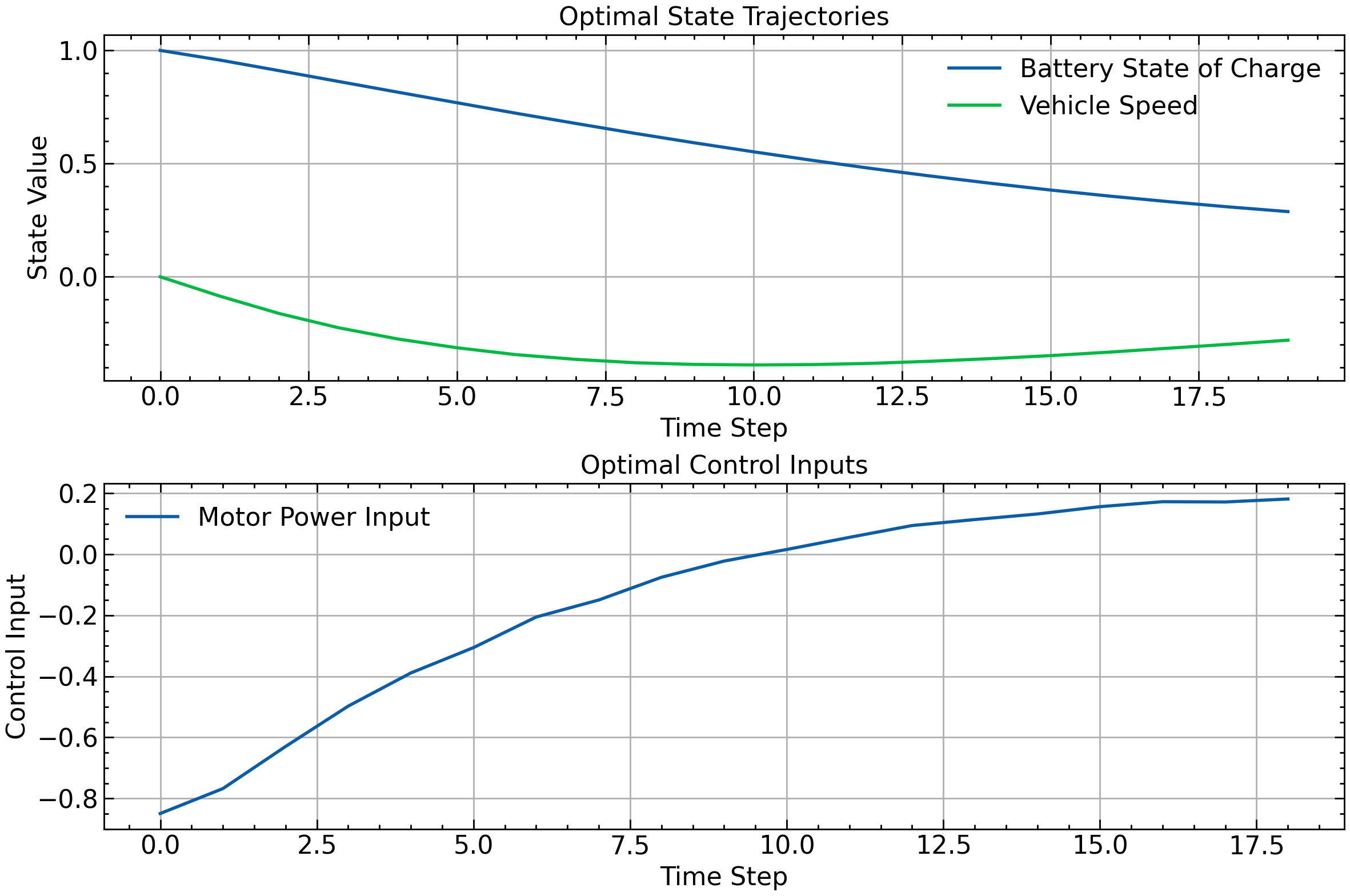
#  label: fig-ocp-single-shooting
#  caption: Single-shooting EV example: the plot shows optimal state trajectories (battery charge and speed) plus the control sequence, while the console reports the optimized control inputs.

%config InlineBackend.figure_format = 'retina'
import jax
import jax.numpy as jnp
from jax import grad, jit
from jax.example_libraries import optimizers
import matplotlib.pyplot as plt

# Apply book style
try:
    import scienceplots
    plt.style.use(['science', 'notebook'])
except (ImportError, OSError):
    pass  # Use matplotlib defaults

def single_shooting_ev_optimization(T=20, num_iterations=1000, step_size=0.01):
    """
    Implements the single shooting method for the electric vehicle energy optimization problem.
    
    Args:
    T: time horizon
    num_iterations: number of optimization iterations
    step_size: step size for the optimizer
    
    Returns:
    optimal_u: optimal control sequence
    """
    
    def f(x, u, t):
        return jnp.array([
            x[0] + 0.1 * x[1] + 0.05 * u,
            x[1] + 0.1 * u
        ])
    
    def c(x, u, t):
        if t == T:
            return x[0]**2 + x[1]**2
        else:
            return 0.1 * (x[0]**2 + x[1]**2 + u**2)
    
    def compute_trajectory_and_cost(u, x1):
        x = x1
        total_cost = 0
        for t in range(1, T):
            total_cost += c(x, u[t-1], t)
            x = f(x, u[t-1], t)
        total_cost += c(x, 0.0, T)  # No control at final step
        return total_cost
    
    def objective(u):
        return compute_trajectory_and_cost(u, x1)
    
    def clip_controls(u):
        return jnp.clip(u, -1.0, 1.0)
    
    x1 = jnp.array([1.0, 0.0])  # Initial state: full battery, zero speed
    
    # Initialize controls
    u_init = jnp.zeros(T-1)
    
    # Setup optimizer
    optimizer = optimizers.adam(step_size)
    opt_init, opt_update, get_params = optimizer
    opt_state = opt_init(u_init)
    
    @jit
    def step(i, opt_state):
        u = get_params(opt_state)
        value, grads = jax.value_and_grad(objective)(u)
        opt_state = opt_update(i, grads, opt_state)
        u = get_params(opt_state)
        u = clip_controls(u)
        opt_state = opt_init(u)
        return value, opt_state
    
    # Run optimization
    for i in range(num_iterations):
        value, opt_state = step(i, opt_state)
        if i % 100 == 0:
            print(f"Iteration {i}, Cost: {value}")
    
    optimal_u = get_params(opt_state)
    return optimal_u

def plot_results(optimal_u, T):
    # Compute state trajectory
    x1 = jnp.array([1.0, 0.0])
    x_trajectory = [x1]
    for t in range(T-1):
        x_next = jnp.array([
            x_trajectory[-1][0] + 0.1 * x_trajectory[-1][1] + 0.05 * optimal_u[t],
            x_trajectory[-1][1] + 0.1 * optimal_u[t]
        ])
        x_trajectory.append(x_next)
    x_trajectory = jnp.array(x_trajectory)

    time = jnp.arange(T)
    
    plt.figure(figsize=(12, 8))
    
    plt.subplot(2, 1, 1)
    plt.plot(time, x_trajectory[:, 0], label='Battery State of Charge')
    plt.plot(time, x_trajectory[:, 1], label='Vehicle Speed')
    plt.xlabel('Time Step')
    plt.ylabel('State Value')
    plt.title('Optimal State Trajectories')
    plt.legend()
    plt.grid(True)
    
    plt.subplot(2, 1, 2)
    plt.plot(time[:-1], optimal_u, label='Motor Power Input')
    plt.xlabel('Time Step')
    plt.ylabel('Control Input')
    plt.title('Optimal Control Inputs')
    plt.legend()
    plt.grid(True)
    
    plt.tight_layout()

# Run the optimization
optimal_u = single_shooting_ev_optimization()
print("Optimal control sequence:", optimal_u)

# Plot the results
plot_results(optimal_u, T=20)

Iteration 0, Cost: 2.9000003337860107
Iteration 100, Cost: 1.4151428937911987
Iteration 200, Cost: 1.4088492393493652
Iteration 300, Cost: 1.4091222286224365
Iteration 400, Cost: 1.409378170967102
Iteration 500, Cost: 1.4096146821975708
Iteration 600, Cost: 1.4098317623138428
Iteration 700, Cost: 1.4100308418273926
Iteration 800, Cost: 1.4102120399475098
Iteration 900, Cost: 1.4103772640228271
Optimal control sequence: [-0.84949344 -0.7677486  -0.62980956 -0.49753863 -0.38879833 -0.30575594
 -0.20555931 -0.14967029 -0.07521405 -0.02217956  0.0158601   0.05557517
  0.0942762   0.11389924  0.13218474  0.15617765  0.17244996  0.17151839
  0.1814026 ]

In Between Sequential and Simultaneous¶

The two formulations we have seen so far lie at opposite ends. The full discretization approach keeps every state explicit and enforces the dynamics through equality constraints, which makes the structure clear but leads to a large optimization problem. At the other end, single shooting removes these constraints by simulating forward from the initial state, leaving only the controls as decision variables. That makes the problem smaller, but it also introduces a long and highly nonlinear dependency from the first control to the last state.

Multiple shooting sits in between. Instead of simulating the entire horizon in one shot, we divide it into smaller segments. For each segment, we keep its starting state as a decision variable and propagate forward using the dynamics for that segment. At the end, we enforce continuity by requiring that the simulated end state of one segment matches the decision variable for the next.

Formally, suppose the horizon of $T$ steps is divided into $K$ segments of length $L$ (with $T = K \cdot L$ for simplicity). We introduce:

• The controls for each step: $\mathbf{u}_{1:T-1}$.

• The state at the start of each segment: $\mathbf{x}_1,\dots,\mathbf{x}_K$.

Given $\mathbf{x}_k$ and the controls in its segment, we compute the predicted terminal state by simulating forward:

where $\Phi$ represents $L$ applications of the dynamics. Continuity constraints enforce:

The resulting nonlinear program looks like this:

Compared to the full NLP, we no longer introduce every intermediate state as a variable, only the anchors at segment boundaries. Inside each segment, states are reconstructed by simulation. Compared to single shooting, these anchors break the long dependency chain that makes optimization unstable: gradients only have to travel across $L$ steps before they hit a decision variable, rather than the entire horizon. This is the same reason why exploding or vanishing gradients appear in deep recurrent networks: when the chain is too long, information either dies out or blows up. Multiple shooting shortens the chain and improves conditioning.

By adjusting the number of segments $K$, we can interpolate between the two extremes: $K = 1$ gives single shooting, while $K = T$ recovers the full direct NLP. In practice, a moderate number of segments often strikes a good balance between robustness and complexity.

#  label: fig-ocp-multiple-shooting
#  caption: Multiple shooting ballistic BVP: the code produces an animation (and optional static plot) that shows how segment defects shrink while steering the projectile to the target.

%config InlineBackend.figure_format = 'retina'
"""
Multiple Shooting as a Boundary-Value Problem (BVP) for a Ballistic Trajectory
-----------------------------------------------------------------------------
We solve for the initial velocities (and total flight time) so that the terminal
position hits a target, enforcing continuity between shooting segments.
"""

import numpy as np
import matplotlib.pyplot as plt

# Apply book style
try:
    import scienceplots
    plt.style.use(['science', 'notebook'])
except (ImportError, OSError):
    pass  # Use matplotlib defaults
from scipy.integrate import solve_ivp
from scipy.optimize import minimize
from IPython.display import HTML, display

# -----------------------------
# Physical parameters
# -----------------------------
g = 9.81          # gravity (m/s^2)
m = 1.0           # mass (kg)
drag_coeff = 0.1  # quadratic drag coefficient


def dynamics(t, state):
    """Ballistic dynamics with quadratic drag. state = [x, y, vx, vy]."""
    x, y, vx, vy = state
    v = np.hypot(vx, vy)
    drag_x = -drag_coeff * v * vx / m if v > 0 else 0.0
    drag_y = -drag_coeff * v * vy / m if v > 0 else 0.0
    dx  = vx
    dy  = vy
    dvx = drag_x
    dvy = drag_y - g
    return np.array([dx, dy, dvx, dvy])


def flow(y0, h):
    """One-segment flow map Φ(y0; h): integrate dynamics over duration h."""
    sol = solve_ivp(dynamics, (0.0, h), y0, method="RK45", rtol=1e-7, atol=1e-9)
    return sol.y[:, -1], sol

# -----------------------------
# Multiple-shooting BVP residuals
# -----------------------------

def residuals(z, K, x_init, x_target):
    """
    Unknowns z = [vx0, vy0, H, y1(4), y2(4), ..., y_{K-1}(4)]  (total len = 3 + 4*(K-1))
    We define y0 from x_init and (vx0, vy0). Each segment has duration h = H/K.
    Residual vector stacks:
      - initial position constraints: y0[:2] - x_init[:2]
      - continuity: y_{k+1} - Φ(y_k; h) for k=0..K-2
      - terminal position constraint at end of last segment: Φ(y_{K-1}; h)[:2] - x_target[:2]
    """
    n = 4
    vx0, vy0, H = z[0], z[1], z[2]
    if H <= 0:
        # Strongly penalize nonpositive durations to keep solver away
        return 1e6 * np.ones(2 + 4*(K-1) + 2)

    h = H / K

    # Build list of segment initial states y_0..y_{K-1}
    ys = []
    y0 = np.array([x_init[0], x_init[1], vx0, vy0], dtype=float)
    ys.append(y0)
    if K > 1:
        rest = z[3:]
        y_internals = rest.reshape(K-1, n)
        ys.extend(list(y_internals))  # y1..y_{K-1}

    res = []

    # Initial position must match exactly
    res.extend(ys[0][:2] - x_init[:2])

    # Continuity across segments
    for k in range(K-1):
        yk = ys[k]
        yk1_pred, _ = flow(yk, h)
        res.extend(ys[k+1] - yk1_pred)

    # Terminal position at the end of last segment equals target
    y_last_end, _ = flow(ys[-1], h)
    res.extend(y_last_end[:2] - x_target[:2])

    # Optional soft "stay above ground" at knots (kept gentle)
    # res.extend(np.minimum(0.0, np.array([y[1] for y in ys])).ravel())

    return np.asarray(res)

# -----------------------------
# Solve BVP via optimization on 0.5*||residuals||^2
# -----------------------------

def solve_bvp_multiple_shooting(K=5, x_init=np.array([0., 0.]), x_target=np.array([10., 0.])):
    """
    K: number of shooting segments.
    x_init: initial position (x0, y0). Initial velocities are unknown.
    x_target: desired terminal position (xT, yT) at time H (unknown).
    """
    # Heuristic initial guesses:
    dx = x_target[0] - x_init[0]
    dy = x_target[1] - x_init[1]
    H0 = max(0.5, dx / 5.0)  # guess ~ 5 m/s horizontal
    vx0_0 = dx / H0
    vy0_0 = (dy + 0.5 * g * H0**2) / H0  # vacuum guess

    # Intentionally disconnected internal knots to visualize defect shrinkage
    internals = []
    for k in range(1, K):  # y1..y_{K-1}
        xk = x_init[0] + (dx * k) / K
        yk = x_init[1] + (dy * k) / K + 2.0  # offset to create mismatch
        internals.append(np.array([xk, yk, 0.0, 0.0]))
    internals = np.array(internals) if K > 1 else np.array([])

    z0 = np.concatenate(([vx0_0, vy0_0, H0], internals.ravel()))

    # Variable bounds: H > 0, keep velocities within a reasonable range
    # Use wide bounds to let the solver work; tune if needed.
    lb = np.full_like(z0, -np.inf, dtype=float)
    ub = np.full_like(z0,  np.inf, dtype=float)
    lb[2] = 1e-2  # H lower bound
    # Optional velocity bounds
    lb[0], ub[0] = -50.0, 50.0
    lb[1], ub[1] = -50.0, 50.0

    # Objective and callback for L-BFGS-B
    def objective(z):
        r = residuals(z, K,
                      np.array([x_init[0], x_init[1], 0., 0.]),
                      np.array([x_target[0], x_target[1], 0., 0.]))
        return 0.5 * np.dot(r, r)

    iterate_history = []
    def cb(z):
        iterate_history.append(z.copy())

    bounds = list(zip(lb.tolist(), ub.tolist()))
    sol = minimize(objective, z0, method='L-BFGS-B', bounds=bounds,
                   callback=cb, options={'maxiter': 300, 'ftol': 1e-12})

    return sol, iterate_history

# -----------------------------
# Reconstruct and plot (optional static figure)
# -----------------------------

def reconstruct_and_plot(sol, K, x_init, x_target):
    n = 4
    vx0, vy0, H = sol.x[0], sol.x[1], sol.x[2]
    h = H / K

    ys = []
    y0 = np.array([x_init[0], x_init[1], vx0, vy0])
    ys.append(y0)
    if K > 1:
        internals = sol.x[3:].reshape(K-1, n)
        ys.extend(list(internals))

    # Integrate each segment and stitch
    traj_x, traj_y = [], []
    for k in range(K):
        yk = ys[k]
        yend, seg = flow(yk, h)
        traj_x.extend(seg.y[0, :].tolist() if k == 0 else seg.y[0, 1:].tolist())
        traj_y.extend(seg.y[1, :].tolist() if k == 0 else seg.y[1, 1:].tolist())

    # Plot
    fig, ax = plt.subplots(figsize=(7, 4.2))
    ax.plot(traj_x, traj_y, '-', label='Multiple-shooting solution')
    ax.plot([x_init[0]], [x_init[1]], 'go', label='Start')
    ax.plot([x_target[0]], [x_target[1]], 'r*', ms=12, label='Target')
    total_pts = len(traj_x)
    for k in range(1, K):
        idx = int(k * total_pts / K)
        ax.axvline(traj_x[idx], color='k', ls='--', alpha=0.3, lw=1)

    ax.set_xlabel('x (m)')
    ax.set_ylabel('y (m)')
    ax.set_title(f'Multiple Shooting BVP (K={K})   H={H:.3f}s   v0=({vx0:.2f},{vy0:.2f}) m/s')
    ax.grid(True, alpha=0.3)
    ax.legend(loc='best')
    plt.tight_layout()

    # Report residual norms
    res = residuals(sol.x, K, np.array([x_init[0], x_init[1], 0., 0.]), np.array([x_target[0], x_target[1], 0., 0.]))
    print(f"\nFinal residual norm: {np.linalg.norm(res):.3e}")
    print(f"vx0={vx0:.4f} m/s, vy0={vy0:.4f} m/s, H={H:.4f} s")

# -----------------------------
# Create JS animation for notebooks
# -----------------------------

def create_animation_progress(iter_history, K, x_init, x_target):
    """Return a JS animation (to_jshtml) showing defect shrinkage across segments."""
    import matplotlib.pyplot as plt
    from matplotlib.animation import FuncAnimation

    # Apply book style
    try:
        import scienceplots
        plt.style.use(['science', 'notebook'])
    except (ImportError, OSError):
        pass  # Use matplotlib defaults

    n = 4

    def unpack(z):
        vx0, vy0, H = z[0], z[1], z[2]
        ys = [np.array([x_init[0], x_init[1], vx0, vy0])]
        if K > 1 and len(z) > 3:
            internals = z[3:].reshape(K-1, n)
            ys.extend(list(internals))
        return H, ys

    fig, ax = plt.subplots(figsize=(7, 4.2))
    ax.set_xlabel('Segment index (normalized time)')
    ax.set_ylabel('y (m)')
    ax.set_title('Multiple Shooting: Defect Shrinkage (Fixed Boundaries)')
    ax.grid(True, alpha=0.3)

    # Start/target markers at fixed indices
    ax.plot([0], [x_init[1]], 'go', label='Start')
    ax.plot([K], [x_target[1]], 'r*', ms=12, label='Target')
    # Vertical dashed lines at boundaries
    for k in range(1, K):
        ax.axvline(k, color='k', ls='--', alpha=0.35, lw=1)
    ax.legend(loc='best')

    # Pre-create line artists
    colors = plt.cm.plasma(np.linspace(0, 1, K))
    segment_lines = [ax.plot([], [], '-', color=colors[k], lw=2, alpha=0.9)[0] for k in range(K)]
    connector_lines = [ax.plot([], [], 'r-', lw=1.4, alpha=0.75)[0] for _ in range(K-1)]

    text_iter = ax.text(0.02, 0.98, '', transform=ax.transAxes,
                        va='top', fontsize=9,
                        bbox=dict(boxstyle='round', facecolor='white', alpha=0.7))

    def animate(i):
        idx = min(i, len(iter_history)-1)
        z = iter_history[idx]
        H, ys = unpack(z)
        h = H / K

        all_y = [x_init[1], x_target[1]]
        total_defect = 0.0
        for k in range(K):
            yk = ys[k]
            yend, seg = flow(yk, h)
            # Map local time to [k, k+1]
            t_local = seg.t
            x_vals = k + (t_local / t_local[-1])
            y_vals = seg.y[1, :]
            segment_lines[k].set_data(x_vals, y_vals)
            all_y.extend(y_vals.tolist())
            if k < K-1:
                y_next = ys[k+1]
                # Vertical connector at boundary x=k+1
                connector_lines[k].set_data([k+1, k+1], [yend[1], y_next[1]])
                total_defect += abs(y_next[1] - yend[1])

        # Fixed x-limits in index space
        ax.set_xlim(-0.1, K + 0.1)
        ymin, ymax = min(all_y), max(all_y)
        margin_y = 0.10 * max(1.0, ymax - ymin)
        ax.set_ylim(ymin - margin_y, ymax + margin_y)

        text_iter.set_text(f'Iterate {idx+1}/{len(iter_history)}  |  Sum vertical defect: {total_defect:.3e}')
        return segment_lines + connector_lines + [text_iter]

    anim = FuncAnimation(fig, animate, frames=len(iter_history), interval=600, blit=False, repeat=True)
    plt.tight_layout()
    js_anim = anim.to_jshtml()
    plt.close(fig)
    return js_anim


def main():
    # Problem definition
    x_init = np.array([0.0, 0.0])      # start at origin
    x_target = np.array([10.0, 0.0])   # hit ground at x=10 m
    K = 6                               # number of shooting segments

    sol, iter_hist = solve_bvp_multiple_shooting(K=K, x_init=x_init, x_target=x_target)
    # Optionally show static reconstruction (commented for docs cleanliness)
    # reconstruct_and_plot(sol, K, x_init, x_target)

    # Animate progression (defect shrinkage across segments) and display as JS
    js_anim = create_animation_progress(iter_hist, K, x_init, x_target)
    display(HTML(js_anim))


if __name__ == "__main__":
    main()

The Discrete-Time Pontryagin Principle¶

If we take the Bolza formulation of the DOCP and apply the KKT conditions directly, we obtain an optimization system with many multipliers and constraints. Written in raw form, it looks like any other nonlinear program. But in control, this structure has a long history and a name of its own: the Pontryagin principle. In fact, the discrete-time version can be seen as the structured KKT system that results from introducing multipliers for the dynamics and collecting terms stage by stage.

We work with the Bolza program

Introduce costates $\boldsymbol{\lambda}_{t+1}\in\mathbb{R}^n$ for the dynamics, multipliers $\boldsymbol{\mu}_t\ge \mathbf{0}$ for path inequalities, and $\boldsymbol{\nu}$ for terminal equalities. The Lagrangian is

It is convenient to package the stagewise terms in a Hamiltonian

Then

Necessary conditions¶

Taking first-order variations and collecting terms gives the discrete-time adjoint system, control stationarity, and complementarity. At a local minimum $\{\mathbf{x}_t^\star,\mathbf{u}_t^\star\}$ with multipliers $\{\boldsymbol{\lambda}_t^\star,\boldsymbol{\mu}_t^\star,\boldsymbol{\nu}^\star\}$:

State dynamics (primal feasibility)

Costate recursion (backward “adjoint” equation)

with the terminal condition

Control stationarity (first-order optimality in $\mathbf{u}_t$) If $\mathcal{U}_t=\mathbb{R}^m$ (no explicit set constraint), then

If $\mathcal{U}_t$ imposes bounds or a convex set, the condition becomes the variational inequality

where $N_{\mathcal{U}_t}(\cdot)$ is the normal cone to $\mathcal{U}_t$. For simple box bounds, this reduces to standard KKT sign and complementarity conditions on the components of $\mathbf{u}_t^\star$.

Path-constraint multipliers (primal/dual feasibility and complementarity)

Terminal equalities (if present)

The triplet “forward state, backward costate, control stationarity” is the discrete-time Euler–Lagrange system tailored to control with dynamics. It is the same KKT logic as before, but organized stagewise through the Hamiltonian.

Recap. The discrete-time Pontryagin principle is the KKT system for trajectory optimization, organized to exploit temporal structure. It has a forward-backward decomposition: states propagate forward through the dynamics, while costates propagate backward through the adjoint equation. The Hamiltonian $H_t$ packages together the stage cost, the dynamics (weighted by the next costate), and any path constraints (weighted by their multipliers). Control stationarity says that optimal controls minimize the Hamiltonian at each stage. Complementarity ensures that only binding constraints carry nonzero multipliers. This structure underlies both analytical solution methods (such as LQR) and numerical algorithms (such as the adjoint method for gradient computation).

The adjoint equation as reverse accumulation¶

Optimization needs sensitivities. In trajectory problems we adjust decisions (controls or parameters) to reduce an objective while respecting dynamics and constraints. First‑order methods in the unconstrained case (e.g., gradient descent, L‑BFGS, Adam) require the gradient of the objective with respect to all controls, and constrained methods (SQP, interior‑point) require gradients of the Lagrangian, i.e., of costs and constraints. The discrete‑time adjoint equations provide these derivatives in a way that scales to long horizons and many decision variables.

Consider

A single forward rollout computes and stores the trajectory $\mathbf{x}_{1:T}$. A single backward sweep then applies the reverse‑mode chain rule stage by stage.

Defining the costate by

yields exactly the discrete‑time adjoint (PMP) recursion.

The gradient with respect to each control follows from the same reverse pass:

Computationally, this reverse accumulation produces all control gradients with one forward rollout and one backward adjoint pass; its cost is essentially a small constant multiple of simulating the system once. Conceptually, the costate $\boldsymbol{\lambda}_t$ is the marginal effect of perturbing the state at time $t$ on the total objective; the control gradient combines a direct contribution from $c_t$ and an indirect contribution through how $\mathbf{u}_t$ changes the next state. This is the same structure that underlies backpropagation, expressed for dynamical systems.

It is instructive to contrast this with alternatives. Black-box finite differences perturb one decision at a time and re-roll the system, requiring on the order of $p$ rollouts for $p$ decision variables and suffering from step-size and noise issues. This becomes prohibitive when $p=(T-1)m$ for an $m$-dimensional control over $T$ steps. Forward‑mode (tangent) sensitivities propagate Jacobian–vector products for each parameter direction; their work also scales with $p$. Reverse‑mode (the adjoint) instead propagates a single vector $\boldsymbol{\lambda}_t$ backward and then reads off all partial derivatives $\nabla_{\mathbf{u}_t} J$ at once. For a scalar objective, its cost is effectively independent of $p$, at the price of storing (or checkpointing) the forward trajectory. This scalability is why the adjoint is the method of choice for gradient‑based trajectory optimization and for constrained transcriptions via the Hamiltonian.

Recap. The adjoint method computes gradients of the objective with respect to all controls in time proportional to a single forward-backward pass through the dynamics. The forward pass simulates the system and stores the trajectory. The backward pass propagates costates $\boldsymbol{\lambda}_t$ from the terminal condition back to the initial time, accumulating sensitivity information along the way. Each control gradient is then read off locally as the sum of a direct cost contribution and an indirect contribution through the dynamics. This is mathematically equivalent to reverse-mode automatic differentiation (backpropagation) applied to the unrolled dynamical system, and it explains why gradient-based trajectory optimization scales gracefully to long horizons and high-dimensional control spaces.

Summary and Outlook¶

This chapter developed the foundations of discrete-time trajectory optimization. We introduced three equivalent formulations of the discrete-time optimal control problem (DOCP)—Bolza, Lagrange, and Mayer—and showed how they reduce to finite-dimensional nonlinear programs once a horizon is fixed.

Three approaches to solving DOCPs were presented, each with distinct trade-offs:

• Simultaneous methods (direct transcription) keep all states and controls as decision variables and enforce the dynamics as equality constraints. This produces a large but sparse NLP whose structure can be exploited by specialized solvers. The explicit state variables anchor the trajectory at every time step, improving robustness and making it straightforward to impose state constraints.

• Sequential methods (single shooting) eliminate state variables by forward simulation, leaving only the controls as decisions. This yields a smaller, unconstrained (or bound-constrained) problem that integrates naturally with automatic differentiation frameworks. The trade-off is sensitivity to initialization and potential numerical instability over long horizons, since errors compound through the dynamics.

• Multiple shooting divides the horizon into segments, treating segment boundaries as decision variables and enforcing continuity between them. This interpolates between the two extremes: it shortens the dependency chains that cause instability in single shooting while avoiding the full size of direct transcription.

The Karush–Kuhn–Tucker (KKT) conditions provide necessary conditions for local optimality in constrained optimization. Applied to the DOCP, they yield the discrete-time Pontryagin principle: a forward-backward system where states propagate forward through the dynamics and costates propagate backward through the adjoint equation. The Hamiltonian packages together the stage cost and dynamics, and control stationarity says that optimal controls minimize the Hamiltonian at each stage.

The adjoint method computes gradients of the objective with respect to all controls in time proportional to one forward pass plus one backward pass, independent of the number of decision variables. This efficiency is what allows gradient-based trajectory optimization to scale to long horizons and high-dimensional control spaces.

The open-loop perspective developed here is foundational but limited: it assumes the model is accurate and that no disturbances will occur. In practice, plans must be adapted as new information arrives. Several directions extend this chapter’s material:

• Collocation methods use polynomial approximations to represent the trajectory between grid points, enabling higher-order accuracy and implicit handling of stiff dynamics. These are the subject of the next chapter.

• Model predictive control (MPC) repeatedly solves trajectory optimization problems in a receding-horizon fashion, using the first control from each solution and re-planning as new state measurements arrive. This creates a feedback policy from open-loop building blocks.

• Feedback and policy optimization shift the focus from computing a single trajectory to learning a policy $\pi(\mathbf{x})$ that maps states to controls. Dynamic programming, policy gradient methods, and actor-critic algorithms address this problem from different angles, and will be developed in later chapters.

The tools introduced here—KKT conditions, the Pontryagin principle, shooting methods, and adjoint gradients—will reappear throughout the book as we move from open-loop planning to closed-loop control and learning.

Exercises¶

Exercise 1: KKT conditions for a simple DOCP¶

Consider a two-stage optimal control problem with scalar state and control:

subject to:

(a) Write out the Lagrangian with multipliers $\lambda_2, \lambda_3$ for the dynamics constraints.

(b) Derive the KKT conditions (stationarity with respect to $x_2, x_3, u_1, u_2$).

(c) Solve the system to find the optimal controls $u_1^\star, u_2^\star$ and the optimal cost.

Exercise 2: Lagrange to Mayer conversion¶

Consider the Lagrange problem:

(a) Introduce an auxiliary state $y_t$ that accumulates the running cost. Write the augmented dynamics and the equivalent Mayer problem.

(b) What is the initial condition for $y_1$? What is the terminal cost in Mayer form?

(c) Verify that the two formulations have the same optimal control sequence.

Exercise 3: When LICQ fails¶

Consider a DOCP where the state must satisfy $x_T = 0$ and also $x_T \leq 0$ at the terminal time.

(a) At a feasible point with $x_T = 0$, which constraints are active?

(b) Write the gradients of the active constraints with respect to $x_T$. Are they linearly independent?

(c) Explain why this violates LICQ and what consequences this might have for the KKT multipliers.

Exercise 4: Costate recursion as sensitivity¶

Consider an unconstrained DOCP with objective $J = c_T(x_T) + \sum_{t=1}^{T-1} c_t(x_t, u_t)$ and dynamics $x_{t+1} = f_t(x_t, u_t)$.

(a) Define the value-to-go from time $t$ as $V_t(x_t) = \min_{u_{t:T-1}} \left[ c_T(x_T) + \sum_{s=t}^{T-1} c_s(x_s, u_s) \right]$. Show that at an optimal trajectory, $\nabla_{x_t} V_t(x_t^\star) = \lambda_t^\star$, where $\lambda_t$ is the costate.