TP5: Mélange d’experts (MoE) - Fondements de l'apprentissage machine

IFT3395/IFT6390 - Fondements de l’apprentissage machine

Ce notebook accompagne le Chapitre 6: Modèles probabilistes génératifs. Il complète le TP3 sur les modèles à variables latentes en présentant le mélange d’experts (MoE), une extension où le rôle de la variable latente dépend de l’entrée.

Objectifs¶

À la fin de ce TP, vous serez en mesure de:

Distinguer le MoE du GMM (routage dépendant de l’entrée vs poids fixes)
Implémenter le réseau de routage (softmax) et les experts (régression linéaire)
Calculer les responsabilités de l’étape E pour le MoE
Mettre à jour les paramètres des experts (régression pondérée)
Mettre à jour les paramètres du routage par maximisation pondérée
Visualiser la spécialisation des experts et la prédiction globale

Prérequis: TP3 (GMM, algorithme EM). Ce TP réutilise les mêmes idées (responsabilités, EM) dans un cadre supervisé de régression.

Partie 0: Configuration¶

Exécutez cette cellule pour importer les bibliothèques nécessaires.

import numpy as np
import matplotlib.pyplot as plt

plt.rcParams['figure.figsize'] = (8, 5)
plt.rcParams['font.size'] = 12

print("Configuration terminée!")

Configuration terminée!

Partie 1: MoE vs GMM¶

Au TP3, le GMM modélise la densité des données $p(\mathbf{x})$ par un mélange où les poids $\pi_k$ sont constants (indépendants de $\mathbf{x}$ ):

p(\mathbf{x}) = \sum_{k=1}^K \pi_k \, \mathcal{N}(\mathbf{x} \mid \boldsymbol{\mu}_k, \boldsymbol{\Sigma}_k)

(1)

Le mélange d’experts (MoE) traite un problème supervisé: étant donné une entrée $\mathbf{x}$ , prédire une sortie $y$ . La différence clé: le réseau de routage $g_k(\mathbf{x}) = p(z=k \mid \mathbf{x})$ dépend de l’entrée. Chaque expert prédit $p(y \mid \mathbf{x}, z=k)$ .

p(y \mid \mathbf{x}) = \sum_{k=1}^K g_k(\mathbf{x}) \, p(y \mid \mathbf{x}, z=k)

(2)

Les experts se spécialisent: chacun gère une région de l’espace d’entrée où il obtient les meilleurs résultats. Le réseau de routage apprend à assigner chaque $\mathbf{x}$ à l’expert approprié.

Partie 2: Données de régression par morceaux¶

Un cas d’utilisation classique du MoE: des données générées par des régimes différents selon la région. Par exemple, une relation $y \approx f(x)$ qui change de pente ou de forme selon $x$ .

Nous générons des données où $y$ suit approximativement deux segments de droite différents selon que $x$ est négatif ou positif.

np.random.seed(42)
n_samples = 200

# Segment 1: x < 0, y ≈ 2x + 1
# Segment 2: x >= 0, y ≈ -1.5x + 2
x = np.random.uniform(-3, 3, n_samples)
noise = np.random.normal(0, 0.3, n_samples)

y = np.where(x < 0, 2 * x + 1, -1.5 * x + 2) + noise

# Ajouter la colonne de biais pour la régression
X = np.column_stack([np.ones(n_samples), x])

print(f"Nombre d'échantillons: {len(x)}")
print(f"x: min={x.min():.2f}, max={x.max():.2f}")
print(f"y: min={y.min():.2f}, max={y.max():.2f}")

Nombre d'échantillons: 200
x: min=-2.97, max=2.92
y: min=-5.08, max=2.69

plt.figure(figsize=(8, 5))
plt.scatter(x, y, c='gray', alpha=0.6, s=25)
plt.axvline(0, color='red', linestyle='--', alpha=0.7, label='Frontière vraie (x=0)')
plt.xlabel('$x$')
plt.ylabel('$y$')
plt.title('Données de régression par morceaux')
plt.legend()
plt.grid(True, alpha=0.3)
plt.tight_layout()
plt.show()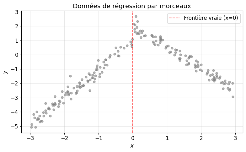

Partie 3: Modèle MoE pour la régression¶

Nous utilisons un MoE avec:

Routage (softmax): $g_k(\mathbf{x}) = \frac{\exp(\mathbf{v}_k^\top \mathbf{x})}{\sum_{j=1}^K \exp(\mathbf{v}_j^\top \mathbf{x})}$ — chaque expert reçoit un poids qui dépend de $\mathbf{x}$ .
Experts (régression linéaire gaussienne): $p(y \mid \mathbf{x}, z=k) = \mathcal{N}(y \mid \mathbf{w}_k^\top \mathbf{x}, \sigma_k^2)$ — l’expert $k$ prédit $y$ par une droite.

La prédiction du modèle est une moyenne pondérée: $\hat{y} = \sum_k g_k(\mathbf{x}) \, \mathbf{w}_k^\top \mathbf{x}$ .

Exercice 1: Fonction de routage softmax ★¶

Complétez la fonction qui calcule $g_k(\mathbf{x})$ pour tous les points et toutes les classes. Utilisez la stabilité numérique: soustrayez le max de chaque ligne avant d’appliquer exp.

def softmax_gating(X, V):
    """
    Calcule les probabilités de routage g_k(x) = softmax(V^T x).

    Args:
        X: entrées avec biais (N, D), chaque ligne = [1, x_1, ..., x_{D-1}]
        V: paramètres du routage (K, D), V[k] = v_k

    Returns:
        g: matrice (N, K), g[n,k] = g_k(x_n)
    """
    # ============================================
    # TODO: logits = X @ V.T  (N, K)
    # Pour la stabilité: logits = logits - logits.max(axis=1, keepdims=True)
    # g = exp(logits) / exp(logits).sum(axis=1, keepdims=True)
    # ============================================
    g = None  # (N, K)
    return g

# Test: V tel que toutes les entrées donnent g ≈ [1/2, 1/2]
V_test = np.array([[0.1, 0.0], [0.1, 0.0]])  # v_1 ≈ v_2
if softmax_gating(X[:3], V_test) is not None:
    g_test = softmax_gating(X[:5], V_test)
    print(f"Somme par ligne (attendu: 1.0): {g_test.sum(axis=1).round(4)}")
    if np.allclose(g_test.sum(axis=1), 1.0):
        print("Correct!")
else:
    print("Complétez softmax_gating!")

Complétez softmax_gating!

def softmax_gating(X, V):
    logits = X @ V.T
    logits = logits - logits.max(axis=1, keepdims=True)
    exp_logits = np.exp(logits)
    g = exp_logits / exp_logits.sum(axis=1, keepdims=True)
    return g

Exercice 2: Prédictions des experts et densité gaussienne ★¶

Chaque expert $k$ prédit $\mu_k(\mathbf{x}) = \mathbf{w}_k^\top \mathbf{x}$ . La densité de $y$ sachant l’expert $k$ est $\mathcal{N}(y \mid \mu_k(\mathbf{x}), \sigma_k^2)$ . Complétez les fonctions.

def expert_predictions(X, weights_list, sigmas):
    """
    Prédictions de chaque expert: mu_k(x) = w_k^T x.

    Args:
        X: (N, D)
        weights_list: liste de K vecteurs w_k (D,)
        sigmas: (K,) variances des experts

    Returns:
        mu: (N, K) prédictions par expert
    """
    K = len(weights_list)
    mu = np.zeros((X.shape[0], K))
    # ============================================
    # TODO: Pour chaque k, mu[:, k] = X @ weights_list[k]
    # ============================================
    return mu


def gaussian_pdf_1d(y, mu, sigma2):
    """Densité gaussienne unidimensionnelle: N(y | mu, sigma2)."""
    # ============================================
    # TODO: (2*pi*sigma2)^{-1/2} * exp(-0.5 * (y-mu)^2 / sigma2)
    # ============================================
    return None  # (N,) si y, mu sont (N,)

def expert_predictions(X, weights_list, sigmas):
    K = len(weights_list)
    mu = np.zeros((X.shape[0], K))
    for k in range(K):
        mu[:, k] = X @ weights_list[k]
    return mu

def gaussian_pdf_1d(y, mu, sigma2):
    norm = 1.0 / np.sqrt(2 * np.pi * sigma2)
    return norm * np.exp(-0.5 * (y - mu) ** 2 / sigma2)

Partie 4: Algorithme EM pour le MoE¶

L’étape E calcule les responsabilités (probabilité a posteriori de l’expert sachant $(\mathbf{x}_n, y_n)$ ):

r_{nk} = \frac{g_k(\mathbf{x}_n) \, \mathcal{N}(y_n \mid \mathbf{w}_k^\top \mathbf{x}_n, \sigma_k^2)}{\sum_{j=1}^K g_j(\mathbf{x}_n) \, \mathcal{N}(y_n \mid \mathbf{w}_j^\top \mathbf{x}_n, \sigma_j^2)}

(3)

L’étape M met à jour:

Experts: régression linéaire pondérée par $r_{nk}$ — formules fermées
Routage: maximisation de $\sum_n \sum_k r_{nk} \log g_k(\mathbf{x}_n)$ — pas de formule fermée pour le softmax; on utilise une descente de gradient

Exercice 3: Étape E — responsabilités ★★¶

Complétez la fonction qui calcule les responsabilités $r_{nk}$ .

def moe_e_step(X, y, V, weights_list, sigmas):
    """
    Étape E: responsabilités r_nk = p(z=k | x_n, y_n).

    Returns:
        responsibilities: (N, K)
    """
    g = softmax_gating(X, V)
    mu = expert_predictions(X, weights_list, sigmas)

    # ============================================
    # TODO: Pour chaque k: likelihood_k = g[:,k] * gaussian_pdf_1d(y, mu[:,k], sigmas[k])
    # responsibilities = likelihood / likelihood.sum(axis=1, keepdims=True)
    # ============================================
    responsibilities = None
    return responsibilities

def moe_e_step(X, y, V, weights_list, sigmas):
    g = softmax_gating(X, V)
    mu = expert_predictions(X, weights_list, sigmas)
    weighted_lik = np.zeros((X.shape[0], len(weights_list)))
    for k in range(len(weights_list)):
        weighted_lik[:, k] = g[:, k] * gaussian_pdf_1d(y, mu[:, k], sigmas[k])
    responsibilities = weighted_lik / weighted_lik.sum(axis=1, keepdims=True)
    return responsibilities

Exercice 4: Étape M — experts (régression pondérée) ★★¶

Pour chaque expert $k$ , la mise à jour est une régression linéaire pondérée: on minimise $\sum_n r_{nk} (y_n - \mathbf{w}_k^\top \mathbf{x}_n)^2$ .

La solution en forme fermée: $\mathbf{w}_k = (\mathbf{X}^\top \mathbf{R}_k \mathbf{X})^{-1} \mathbf{X}^\top \mathbf{R}_k \mathbf{y}$ , où $\mathbf{R}_k = \text{diag}(r_{1k}, \ldots, r_{Nk})$ .

La variance: $\sigma_k^2 = \frac{\sum_n r_{nk} (y_n - \mathbf{w}_k^\top \mathbf{x}_n)^2}{\sum_n r_{nk}}$

def moe_m_step_experts(X, y, responsibilities):
    """
    Étape M: met à jour les paramètres des experts (w_k, sigma_k^2).

    Returns:
        weights_list: liste de K vecteurs (D,)
        sigmas: (K,)
    """
    N, D = X.shape
    K = responsibilities.shape[1]
    weights_list = []
    sigmas = np.zeros(K)

    for k in range(K):
        r_k = responsibilities[:, k]  # (N,)
        N_k = r_k.sum()
        # ============================================
        # TODO: X_weighted = sqrt(r_k) * X  (pondérer les lignes)
        #       y_weighted = sqrt(r_k) * y
        # w_k = solution de (X_weighted^T X_weighted) w = X_weighted^T y_weighted
        # Ou: w_k = (X^T R_k X)^{-1} X^T (r_k * y)  avec R_k = diag(r_k)
        # ============================================
        # w_k = np.linalg.solve(X.T @ np.diag(r_k) @ X, X.T @ (r_k * y))
        # Ou plus efficace: X_r = np.sqrt(r_k)[:, None] * X, y_r = np.sqrt(r_k) * y
        # w_k = np.linalg.lstsq(X_r, y_r, rcond=None)[0]
        w_k = None  # <- Complétez
        weights_list.append(w_k)

        # Variance
        pred_k = X @ w_k
        sigmas[k] = np.sum(r_k * (y - pred_k) ** 2) / N_k + 1e-6

    return weights_list, sigmas

def moe_m_step_experts(X, y, responsibilities):
    N, D = X.shape
    K = responsibilities.shape[1]
    weights_list = []
    sigmas = np.zeros(K)

    for k in range(K):
        r_k = responsibilities[:, k]
        N_k = r_k.sum()
        X_r = np.sqrt(r_k)[:, np.newaxis] * X
        y_r = np.sqrt(r_k) * y
        w_k = np.linalg.lstsq(X_r, y_r, rcond=None)[0]
        weights_list.append(w_k)
        pred_k = X @ w_k
        sigmas[k] = np.sum(r_k * (y - pred_k) ** 2) / N_k + 1e-6

    return weights_list, sigmas

Exercice 5: Étape M — routage ★★★¶

On maximise $\mathcal{L}(\mathbf{V}) = \sum_n \sum_k r_{nk} \log g_k(\mathbf{x}_n)$ . Le gradient par rapport à $\mathbf{v}_k$ est:

\nabla_{\mathbf{v}_k} \mathcal{L} = \sum_n (r_{nk} - g_k(\mathbf{x}_n)) \, \mathbf{x}_n

(4)

Complétez la mise à jour du routage par quelques itérations de montée du gradient (ou utilisez scipy.optimize).

def moe_m_step_gating(X, responsibilities, V_init, n_steps=50, lr=0.1):
    """
    Étape M: met à jour V par montée du gradient sur la log-vraisemblance pondérée.

    Returns:
        V: (K, D)
    """
    V = V_init.copy()
    for _ in range(n_steps):
        g = softmax_gating(X, V)
        # ============================================
        # TODO: Pour chaque k: grad_vk = X.T @ (r[:,k] - g[:,k])
        # V = V + lr * grad
        # ============================================
        for k in range(V.shape[0]):
            grad_k = None  # <- Complétez
            V[k] = V[k] + lr * grad_k
    return V

def moe_m_step_gating(X, responsibilities, V_init, n_steps=50, lr=0.1):
    V = V_init.copy()
    for _ in range(n_steps):
        g = softmax_gating(X, V)
        for k in range(V.shape[0]):
            grad_k = X.T @ (responsibilities[:, k] - g[:, k])
            V[k] = V[k] + lr * grad_k
    return V

Exercice 6: Algorithme EM complet ★★¶

Assemblez l’algorithme EM en alternant les étapes E et M.

def moe_em(X, y, K=2, n_iterations=30, seed=42):
    """
    EM pour mélange d'experts.

    Returns:
        V, weights_list, sigmas: paramètres
        responsibilities: (N, K)
        log_likelihoods: liste
    """
    N, D = X.shape
    np.random.seed(seed)

    # Initialisation
    V = np.random.randn(K, D) * 0.1
    indices = np.random.choice(N, K, replace=False)
    weights_list = [np.linalg.lstsq(X, y, rcond=None)[0] + np.random.randn(D) * 0.1 for _ in range(K)]
    sigmas = np.ones(K) * 0.5

    log_likelihoods = []

    for t in range(n_iterations):
        # Étape E
        responsibilities = None  # <- moe_e_step(...)

        # Étape M
        weights_list, sigmas = None, None  # <- moe_m_step_experts(...)
        V = None  # <- moe_m_step_gating(...)

        # Log-vraisemblance
        g = softmax_gating(X, V)
        mu = expert_predictions(X, weights_list, sigmas)
        weighted_pdf = np.zeros(N)
        for k in range(K):
            weighted_pdf += g[:, k] * gaussian_pdf_1d(y, mu[:, k], sigmas[k])
        log_likelihoods.append(np.sum(np.log(weighted_pdf + 1e-10)))

    return V, weights_list, sigmas, responsibilities, log_likelihoods

def moe_em(X, y, K=2, n_iterations=30, seed=42):
    N, D = X.shape
    np.random.seed(seed)

    V = np.random.randn(K, D) * 0.1
    weights_list = [np.linalg.lstsq(X, y, rcond=None)[0] + np.random.randn(D) * 0.1 for _ in range(K)]
    sigmas = np.ones(K) * 0.5
    log_likelihoods = []

    for t in range(n_iterations):
        responsibilities = moe_e_step(X, y, V, weights_list, sigmas)
        weights_list, sigmas = moe_m_step_experts(X, y, responsibilities)
        V = moe_m_step_gating(X, responsibilities, V, n_steps=50, lr=0.1)

        g = softmax_gating(X, V)
        mu = expert_predictions(X, weights_list, sigmas)
        log_lik = 0.0
        for n in range(N):
            mix = sum(g[n, k] * gaussian_pdf_1d(np.array([y[n]]), np.array([mu[n, k]]), sigmas[k])[0] for k in range(K))
            log_lik += np.log(mix + 1e-10)
        log_likelihoods.append(log_lik)

    return V, weights_list, sigmas, responsibilities, log_likelihoods

# Exécuter EM
V_moe, w_moe, sig_moe, resp_moe, ll_moe = moe_em(X, y, K=2, n_iterations=30, seed=42)

if resp_moe is not None and len(ll_moe) > 0:
    print("Paramètres appris:")
    for k in range(2):
        print(f"  Expert {k+1}: w = [{w_moe[k][0]:.3f}, {w_moe[k][1]:.3f}], sigma^2 = {sig_moe[k]:.4f}")
    print(f"\nLog-vraisemblance: {ll_moe[0]:.1f} -> {ll_moe[-1]:.1f}")
else:
    print("Complétez moe_em!")

---------------------------------------------------------------------------
TypeError                                 Traceback (most recent call last)
Cell In[11], line 2
      1 # Exécuter EM
----> 2 V_moe, w_moe, sig_moe, resp_moe, ll_moe = moe_em(X, y, K=2, n_iterations=30, seed=42)
      4 if resp_moe is not None and len(ll_moe) > 0:
      5     print("Paramètres appris:")

Cell In[10], line 31, in moe_em(X, y, K, n_iterations, seed)
     29 # Log-vraisemblance
     30 g = softmax_gating(X, V)
---> 31 mu = expert_predictions(X, weights_list, sigmas)
     32 weighted_pdf = np.zeros(N)
     33 for k in range(K):

Cell In[6], line 13, in expert_predictions(X, weights_list, sigmas)
      1 def expert_predictions(X, weights_list, sigmas):
      2     """
      3     Prédictions de chaque expert: mu_k(x) = w_k^T x.
      4 
   (...)     11         mu: (N, K) prédictions par expert
     12     """
---> 13     K = len(weights_list)
     14     mu = np.zeros((X.shape[0], K))
     15     # ============================================
     16     # TODO: Pour chaque k, mu[:, k] = X @ weights_list[k]
     17     # ============================================

TypeError: object of type 'NoneType' has no len()

Partie 5: Visualisation¶

Visualisons la spécialisation des experts: chaque expert prédit une droite; le routage détermine quel expert domine dans quelle région.

def moe_predict(X, V, weights_list, sigmas):
    """Prédiction du MoE: y_hat = sum_k g_k(x) * w_k^T x."""
    g = softmax_gating(X, V)
    mu = expert_predictions(X, weights_list, sigmas)
    return (g * mu).sum(axis=1)

if resp_moe is not None:
    x_grid = np.linspace(x.min(), x.max(), 200)
    X_grid = np.column_stack([np.ones(200), x_grid])

    g_grid = softmax_gating(X_grid, V_moe)
    mu_grid = expert_predictions(X_grid, w_moe, sig_moe)
    y_pred = moe_predict(X_grid, V_moe, w_moe, sig_moe)

    fig, axes = plt.subplots(1, 2, figsize=(12, 5))

    ax = axes[0]
    ax.scatter(x, y, c='gray', alpha=0.5, s=20)
    ax.plot(x_grid, mu_grid[:, 0], 'C0-', linewidth=2, label='Expert 1')
    ax.plot(x_grid, mu_grid[:, 1], 'C1-', linewidth=2, label='Expert 2')
    ax.plot(x_grid, y_pred, 'k--', linewidth=2, label='Prédiction MoE')
    ax.set_xlabel('$x$')
    ax.set_ylabel('$y$')
    ax.set_title('Experts et prédiction globale')
    ax.legend()
    ax.grid(True, alpha=0.3)

    ax = axes[1]
    ax.plot(x_grid, g_grid[:, 0], 'C0-', linewidth=2, label='$g_1(x)$')
    ax.plot(x_grid, g_grid[:, 1], 'C1-', linewidth=2, label='$g_2(x)$')
    ax.set_xlabel('$x$')
    ax.set_ylabel('Poids du routage')
    ax.set_title('Réseau de routage: quel expert domine?')
    ax.legend()
    ax.grid(True, alpha=0.3)
    ax.set_ylim(-0.05, 1.05)

    plt.tight_layout()
    plt.show()
else:
    print("Complétez d'abord l'algorithme EM!")

Questions de réflexion:

Comment le routage $g_1(x)$ et $g_2(x)$ se comportent-ils autour de $x=0$ ? Pourquoi?
En quoi le MoE diffère-t-il d’une simple régression linéaire sur ces données?
Dans un GMM, les poids $\pi_k$ ne dépendent pas de $\mathbf{x}$ . Quelle conséquence cela a-t-il pour des données de régression?

Partie 6: MoE vs régression linéaire ★¶

Comparons l’erreur de prédiction du MoE avec une régression linéaire unique.

if resp_moe is not None:
    y_pred_moe = moe_predict(X, V_moe, w_moe, sig_moe)
    mse_moe = np.mean((y - y_pred_moe) ** 2)

    w_linear = np.linalg.lstsq(X, y, rcond=None)[0]
    y_pred_linear = X @ w_linear
    mse_linear = np.mean((y - y_pred_linear) ** 2)

    print("Comparaison (erreur quadratique moyenne sur les données d'entraînement):")
    print(f"  Régression linéaire: {mse_linear:.4f}")
    print(f"  MoE (2 experts):    {mse_moe:.4f}")
else:
    print("Complétez l'algorithme EM!")

Récapitulatif¶

Le mélange d’experts (MoE) généralise l’idée du GMM au cadre supervisé:

Aspect	GMM	MoE
Problème	Non supervisé (densité $p(\mathbf{x})$ )	Supervisé (régression $p(y \mid \mathbf{x})$ )
Poids	$\pi_k$ constants	$g_k(\mathbf{x})$ dépendent de l’entrée
Variable latente	$p(z=k) = \pi_k$	$p(z=k \mid \mathbf{x}) = g_k(\mathbf{x})$

Le réseau de routage apprend à aiguiller chaque entrée vers l’expert le plus compétent. L’algorithme EM alterne le calcul des responsabilités (étape E) et la mise à jour des experts et du routage (étape M). Les experts deviennent des experts locaux spécialisés dans différentes régions de l’espace d’entrée.

Pour aller plus loin: Chapitre 6: Modèles probabilistes génératifs, TP3 (GMM)