TP6: Dérivée totale, VJP et différentiation automatique

IFT3395/IFT6390 — Fondements de l’apprentissage machine

Ce notebook accompagne le Chapitre 7: Réseaux de neurones, sections « Rétropropagation » et « Différentiation automatique ». Vous y dériverez des règles VJP à la main, puis les vérifierez numériquement avec JAX.

Objectifs¶

À la fin de ce TP, vous serez en mesure de:

• Interpréter la dérivée totale $Df(\mathbf{a})$ comme une application linéaire, pas une matrice

• Relier les dérivées partielles aux restrictions de $Df(\mathbf{a})$ (projections et injections)

• Appliquer la règle de la chaîne comme composition d’applications linéaires

• Calculer des JVP et VJP avec JAX et vérifier par différences finies

• Dériver des règles VJP à la main pour des opérations courantes

• Composer des VJP pour rétropropager un gradient à travers une chaîne de fonctions

• Comparer le coût computationnel du mode avant (JVP) et du mode arrière (VJP)

Prérequis: Ch7, sections « Rétropropagation » et « Différentiation automatique » (en particulier le tableau des règles VJP et l’implémentation minimale avec Var/grad).

Partie 0: Configuration¶

Exécutez cette cellule pour importer les bibliothèques nécessaires. Si vous utilisez Colab, JAX est déjà installé. Localement: pip install jax.

Partie 1: La notation de Spivak — pourquoi et comment¶

Avant de plonger dans les calculs, clarifions la notation utilisée dans ce TP. Elle diffère peut-être de celle de vos cours de calcul, mais elle a des avantages concrets pour la suite.

Deux traditions de notation¶

La notation de Leibniz — $\frac{\partial y}{\partial x}$, $\frac{\partial f}{\partial x_j}$ — est un raccourci commode, mais elle masque un fait important: la dérivée est une fonction (un opérateur), pas un nombre ni un rapport. Quand on écrit $\frac{\partial f}{\partial x_1}$, on ne voit pas immédiatement que le résultat dépend du point d’évaluation, ni que la « vraie » dérivée est un objet plus riche qu’une collection de dérivées partielles.

La notation de Spivak adopte une autre perspective: $Df(\mathbf{a})$ désigne la dérivée de la fonction $f$, évaluée au point $\mathbf{a}$. Le résultat est une application linéaire — une fonction qui prend un vecteur et renvoie un vecteur. Pas d’ambiguïté sur ce qu’on dérive ni où.

Pourquoi l’adopter ici¶

Trois raisons pratiques:

1. Elle correspond à JAX. L’appel jax.jvp(f, (a,), (v,)) applique littéralement l’application linéaire $Df(\mathbf{a})$ au vecteur $\mathbf{v}$. La fonction f est le premier argument, le point $\mathbf{a}$ le deuxième, la direction $\mathbf{v}$ le troisième. Pas de « $\partial$ sortie / $\partial$ entrée » — juste: fonction, point, direction.

2. La règle de la chaîne devient limpide. $D(g \circ f)(\mathbf{a}) = Dg(f(\mathbf{a})) \circ Df(\mathbf{a})$: c’est une composition de fonctions. Pas de $\Sigma$, pas d’indices, pas de conventions d’appariement.

3. Elle passe à l’échelle. La même écriture fonctionne pour des scalaires, des vecteurs, des matrices ou des tenseurs, sans changer de convention.

Tableau de référence¶

Gardez ce tableau sous la main pour le reste du TP:

La perspective opérateur¶

$D$ est un opérateur qui transforme une fonction en une nouvelle fonction:

Ensuite, $Df(\mathbf{a})$ est l’application linéaire obtenue en évaluant $Df$ au point $\mathbf{a}$. Enfin, $Df(\mathbf{a})(\mathbf{v})$ est cette application linéaire appliquée au vecteur $\mathbf{v}$. Trois niveaux d’« application de fonction » — et chacun correspond à un appel JAX:

Partie 2: La dérivée totale comme application linéaire¶

En calcul à une variable, on écrit $f'(a) \in \mathbb{R}$: la dérivée est un nombre. En plusieurs variables, la situation est plus riche. Plutôt qu’une matrice de dérivées partielles, la notion fondamentale est celle d’application linéaire.

Définition (Spivak). Soit $f: \mathbb{R}^n \to \mathbb{R}^m$. La dérivée totale de $f$ en $\mathbf{a}$ est l’unique application linéaire $Df(\mathbf{a}): \mathbb{R}^n \to \mathbb{R}^m$ telle que

Trois points à retenir:

1. $Df(\mathbf{a})$ est une fonction — elle prend un vecteur $\mathbf{v} \in \mathbb{R}^n$ et renvoie un vecteur $Df(\mathbf{a})(\mathbf{v}) \in \mathbb{R}^m$.

2. La matrice jacobienne $\mathbf{J}_f(\mathbf{a}) \in \mathbb{R}^{m \times n}$ représente cette application linéaire dans la base canonique: $Df(\mathbf{a})(\mathbf{v}) = \mathbf{J}_f(\mathbf{a}) \, \mathbf{v}$.

3. L’écriture $Df(\mathbf{a})(\mathbf{v})$ est exactement ce que JAX appelle un JVP (Jacobian-vector product).

Travaillons avec un exemple concret tout au long du TP.

Exemple fil conducteur. Considérons $f: \mathbb{R}^2 \to \mathbb{R}^3$ définie par

évaluée au point $\mathbf{a} = (1, 2)$. La jacobienne vaut

Maintenant, appliquons $Df(\mathbf{a})$ en tant que fonction à un vecteur tangent $\mathbf{v} = (0{,}5,\; -1)$. On peut le faire de deux façons:

1. Produit matrice-vecteur: $\mathbf{J}_f(\mathbf{a}) \, \mathbf{v}$ (forme la matrice, puis multiplie)

2. jax.jvp: calcule $Df(\mathbf{a})(\mathbf{v})$ directement, sans former la matrice

Les deux donnent le même résultat — mais jax.jvp est plus efficace car il ne matérialise jamais la jacobienne.

Exercice 1: Vérification de la définition de Spivak ★¶

La définition exige que l’erreur d’approximation linéaire décroisse plus vite que $\|\mathbf{h}\|$. En posant $\mathbf{h} = t \, \mathbf{v}$ pour un $\mathbf{v}$ fixé, le rapport

doit tendre vers 0 quand $t \to 0$. Plus précisément, on s’attend à $r(t) = O(t)$ pour une fonction lisse (l’erreur est dominée par le terme quadratique).

Complétez le code ci-dessous pour vérifier cette propriété numériquement, puis tracez $r(t)$ en échelle log-log.

Partie 3: Dérivées partielles comme restrictions¶

On écrit souvent $\frac{\partial f_i}{\partial x_j}(\mathbf{a})$ comme si c’était une quantité primitive. En réalité, cette dérivée partielle est une restriction de la dérivée totale $Df(\mathbf{a})$. Deux opérations la définissent:

• Injection $\iota_j: \mathbb{R} \to \mathbb{R}^n$, qui envoie un scalaire $t$ sur le vecteur $t \, \mathbf{e}_j$ (perturbation le long de l’axe $j$ uniquement)

• Projection $\pi_i: \mathbb{R}^m \to \mathbb{R}$, qui extrait la composante $i$: $\pi_i(\mathbf{y}) = y_i$

La dérivée partielle est alors la composition

Autrement dit: on injecte un vecteur unitaire $\mathbf{e}_j$ dans la dérivée totale, puis on projette sur la composante $i$. Les entrées de la jacobienne ne sont pas la définition — elles en sont une conséquence.

En code, $\iota_j(1) = \mathbf{e}_j$ est simplement un vecteur canonique, et $\pi_i$ est l’indexation [i].

Exercice 2: Reconstruire la jacobienne colonne par colonne (JVP) ★¶

Un JVP $Df(\mathbf{a})(\mathbf{e}_j)$ donne la $j$-ième colonne de $\mathbf{J}_f(\mathbf{a})$: c’est le vecteur des réponses de toutes les sorties à une perturbation unitaire de l’entrée $j$.

Reconstruisez la jacobienne $\mathbf{J}_f(\mathbf{a})$ colonne par colonne en utilisant $n = 2$ appels à jax.jvp, un par vecteur canonique $\mathbf{e}_j$.

Exercice 3: Reconstruire la jacobienne ligne par ligne (VJP) ★★¶

Le VJP offre une vue duale. Rappelons que jax.vjp(f, a) renvoie (f(a), vjp_fn) où vjp_fn(u) calcule $\mathbf{J}_f(\mathbf{a})^\top \mathbf{u}$.

Si on choisit $\mathbf{u} = \mathbf{e}_i$ (vecteur canonique de $\mathbb{R}^m$), on obtient

Reconstruisez la jacobienne ligne par ligne en utilisant $m = 3$ appels VJP.

Observation clé: l’exercice 2 utilise $n$ JVP (un par entrée), celui-ci utilise $m$ VJP (un par sortie). Lequel est plus économique dépend de $n$ et $m$.

Partie 4: Règle de la chaîne — composition d’applications linéaires¶

Dans la notation de Spivak, la règle de la chaîne s’écrit

C’est une composition d’applications linéaires, pas un « produit de dérivées ». En coordonnées, cela donne le produit de matrices jacobiennes:

Définissons une seconde fonction pour composer avec $f$:

Exercice 4: Trois façons de calculer la jacobienne d’une composition ★★¶

Calculez $\mathbf{J}_h(\mathbf{a})$ de trois manières et vérifiez qu’elles coïncident:

1. Directement: jax.jacobian(h)(a)

2. Produit de jacobiennes: $\mathbf{J}_g(f(\mathbf{a})) \cdot \mathbf{J}_f(\mathbf{a})$

3. Composition de JVP: pour chaque $\mathbf{e}_j$, calculer $Dg(f(\mathbf{a}))\bigl(Df(\mathbf{a})(\mathbf{e}_j)\bigr)$ par deux appels imbriqués à jax.jvp

Partie 5: Le produit vecteur-jacobienne (VJP)¶

La dérivée totale $Df(\mathbf{a})$ est une application linéaire représentée par la matrice jacobienne $\mathbf{J}_f(\mathbf{a}) \in \mathbb{R}^{m \times n}$. Le JVP multiplie cette matrice par un vecteur à droite: $\mathbf{J} \mathbf{v}$.

Le VJP (vector-Jacobian product) effectue l’opération duale: on prend un vecteur $\mathbf{u} \in \mathbb{R}^m$ et on le multiplie à gauche de la jacobienne:

Le résultat est un vecteur de $\mathbb{R}^n$, de la même taille que l’entrée de $f$. Le vecteur $\mathbf{u}$ est appelé cotangent. Il représente un signal qui arrive de la sortie, et le VJP le traduit vers l’entrée. En rétropropagation, chaque couche reçoit un cotangent et le propage en arrière grâce à son VJP.

En JAX, jax.vjp(f, a) renvoie (f(a), vjp_fn), et vjp_fn(u) calcule $\mathbf{u}^\top \mathbf{J}_f(\mathbf{a})$.

Dans certains manuels, le VJP est écrit $\mathbf{J}^\top \mathbf{u}$ (transposer la matrice puis multiplier à droite) plutôt que $\mathbf{u}^\top \mathbf{J}$ (multiplier à gauche). Les deux donnent le même vecteur. La seconde écriture évite de transposer et correspond littéralement au nom vector-Jacobian product. En algèbre linéaire, cette opération est l’adjoint de $Df(\mathbf{a})$, noté $[Df(\mathbf{a})]^*$.

Méthode systématique pour dériver une règle VJP¶

Le VJP d’une fonction $f$ au point $\mathbf{a}$ est le produit $\mathbf{u}^\top \mathbf{J}_f(\mathbf{a})$. On pourrait calculer $\mathbf{J}$ en entier puis effectuer le produit matriciel, mais la jacobienne est souvent trop grande pour être stockée. On cherche donc à écrire $\mathbf{u}^\top \mathbf{J}$ sans former la matrice. Pour beaucoup d’opérations courantes, le résultat se réduit à quelques multiplications élément par élément.

Recette en 3 étapes pour toute opération $f: \mathbb{R}^n \to \mathbb{R}^m$:

1. Calculer les dérivées partielles $\frac{\partial f_i}{\partial x_j}(\mathbf{a})$ et les organiser dans la matrice $\mathbf{J} \in \mathbb{R}^{m \times n}$.

2. Calculer $\mathbf{u}^\top \mathbf{J}$. La $j$-ième composante du résultat est $\displaystyle\sum_i u_i \frac{\partial f_i}{\partial x_j}(\mathbf{a})$.

3. Simplifier: chercher une formule directe (produit élément par élément, produit matrice-vecteur, etc.) qui donne le même résultat sans construire la matrice.

Deux exemples avec des valeurs numériques illustrent cette recette.

Exemple A: exponentielle élément par élément¶

Soit $f(\mathbf{x}) = e^{\mathbf{x}}$, c’est-à-dire $f_i(\mathbf{x}) = e^{x_i}$. Prenons $\mathbf{a} = (1, 2, 0)$ et $\mathbf{u} = (0{,}5,\; -1,\; 2)$.

Étape 1. Chaque sortie $f_i$ ne dépend que de $x_i$, donc les dérivées hors-diagonale sont nulles:

Étape 2. On multiplie le vecteur ligne $\mathbf{u}^\top$ par chaque colonne de $\mathbf{J}$. Puisque $\mathbf{J}$ est diagonale, chaque colonne n’a qu’une entrée non nulle:

Étape 3. Chaque composante du résultat est $u_j \cdot e^{a_j}$, ce qui donne une multiplication élément par élément:

Le coût est $O(n)$ au lieu de $O(n^2)$ si on avait formé la matrice entière.

Exemple B: somme (réduction)¶

Soit $f(\mathbf{x}) = \sum_i x_i$, qui prend un vecteur de $n$ nombres et renvoie un scalaire. Prenons $\mathbf{a} = (3, -1, 4)$ et $u = 5$. Ici $\mathbf{u}$ est un scalaire puisque la sortie l’est aussi.

Étape 1. La sortie est un scalaire, donc la jacobienne est un vecteur ligne:

Étape 2. Un scalaire fois un vecteur ligne:

Étape 3. Le scalaire $u$ est copié sur chaque composante:

La somme contracte $n$ valeurs en une seule; son VJP fait l’inverse et diffuse le scalaire $u$ en $n$ copies. Ce patron réduction/diffusion revient constamment en rétropropagation.

Les exercices suivants appliquent cette même recette à trois opérations plus riches.

Exercice 5: Dériver et vérifier des règles VJP ★★¶

Appliquez la recette en 4 étapes pour dériver la règle VJP de chaque opération ci-dessous, puis vérifiez numériquement en implémentant la formule manuelle et en comparant avec jax.vjp.

(a) Carré élément par élément: $\varphi(\mathbf{x}) = \mathbf{x}^{\odot 2}$

La jacobienne est $D\varphi(\mathbf{a}) = \operatorname{diag}(2\mathbf{a})$. La règle VJP:

(b) Produit matrice-vecteur: $f(\mathbf{z}) = W\mathbf{z}$ avec $W \in \mathbb{R}^{m \times n}$ fixe.

La jacobienne par rapport à $\mathbf{z}$ est $Df(\mathbf{a}) = W$ (application linéaire constante). La règle VJP:

(c) ★★★ Softmax: $\sigma: \mathbb{R}^K \to \mathbb{R}^K$, $\sigma_i(\mathbf{a}) = \frac{e^{a_i}}{\sum_j e^{a_j}}$.

La jacobienne a pour entrées $\frac{\partial \sigma_i}{\partial a_j} = \sigma_i(\delta_{ij} - \sigma_j)$, ce qui donne la règle VJP:

Ce concept est subtil. Prenez le temps de dérouler le produit $\mathbf{J}_\sigma^\top \mathbf{u}$ à la main pour voir comment cette formule émerge.

Exercice 6: Gradients par composition de VJP ★★¶

L’exercice 5 a établi les règles VJP pour des opérations individuelles. Ici, on pratique la compétence complémentaire: décomposer une fonction scalaire en chaîne de primitives, puis composer les VJP en ordre inverse pour obtenir le gradient.

La méthode est toujours la même. Soit $\ell = h_k \circ \cdots \circ h_1$:

1. Passe avant: identifier les valeurs intermédiaires $\mathbf{z}_0 = \mathbf{a}$, $\mathbf{z}_1 = h_1(\mathbf{z}_0)$, ..., $\mathbf{z}_k = \ell$.

2. Passe arrière: partir de $\bar{\mathbf{z}}_k = 1$ (cotangent initial pour une perte scalaire) et propager: $\bar{\mathbf{z}}_{i-1} = [Dh_i(\mathbf{z}_{i-1})]^*(\bar{\mathbf{z}}_i)$.

3. Le gradient est $\nabla \ell(\mathbf{a}) = \bar{\mathbf{z}}_0$.

Dérivez le gradient sur papier en composant les règles VJP de l’exercice 5, puis vérifiez avec jax.grad.

(a) ★ Norme au carré: $\ell(\mathbf{x}) = \sum_i x_i^2$

Décomposition: $\mathbf{x} \xrightarrow{(\cdot)^2} \mathbf{x}^{\odot 2} \xrightarrow{\sum} \ell$

(b) ★★ Log-sum-exp: $\ell(\mathbf{x}) = \log\bigl(\sum_i e^{x_i}\bigr)$

Décomposition: $\mathbf{x} \xrightarrow{\exp} \mathbf{y} \xrightarrow{\sum} S \xrightarrow{\log} \ell$

(c) ★★ Moindres carrés: $\ell(\mathbf{x}) = \|A\mathbf{x} - \mathbf{b}\|^2$ avec $A \in \mathbb{R}^{m \times n}$ et $\mathbf{b} \in \mathbb{R}^m$ fixes.

Décomposition: $\mathbf{x} \xrightarrow{A \cdot} \mathbf{z} \xrightarrow{- \mathbf{b}} \mathbf{r} \xrightarrow{(\cdot)^2} \mathbf{r}^{\odot 2} \xrightarrow{\sum} \ell$

(d) ★★★ Entropie croisée: $\ell(\mathbf{z}) = -\log\bigl(\sigma(\mathbf{z})_k\bigr)$ avec $k$ la classe cible et $\sigma$ le softmax.

Décomposition: $\mathbf{z} \xrightarrow{\sigma} \boldsymbol{\sigma} \xrightarrow{\pi_k} \sigma_k \xrightarrow{-\log} \ell$

Partie 6: Composition de VJP et coût computationnel¶

En prenant l’adjoint de la règle de la chaîne $D(g \circ f)(\mathbf{a}) = Dg(f(\mathbf{a})) \circ Df(\mathbf{a})$, et en utilisant $(AB)^\top = B^\top A^\top$, on obtient

L’ordre s’inverse: on applique d’abord l’adjoint de la fonction extérieure $g$, puis celui de la fonction intérieure $f$. C’est la rétropropagation: le signal $\mathbf{u}$ se propage de la sortie vers l’entrée.

Pourquoi le nombre de passes dépend des dimensions¶

Rappelons les exercices 2 et 3: un JVP avec $\mathbf{e}_j$ donne la colonne $j$ de la jacobienne, un VJP avec $\mathbf{e}_i$ donne la ligne $i$. Pour reconstruire la jacobienne complète $\mathbf{J} \in \mathbb{R}^{m \times n}$, il faut donc:

• $n$ passes JVP (une par colonne), ou

• $m$ passes VJP (une par ligne)

Voyons ce que cela donne concrètement sur un petit exemple.

Le tableau suivant résume le nombre de passes nécessaires pour différentes configurations:

Règle générale: le mode arrière (VJP) domine quand $m \ll n$. En apprentissage machine, la perte est toujours scalaire ($m = 1$) et le nombre de paramètres est grand ($n \gg 1$). C’est pourquoi la rétropropagation — qui est une composition de VJP — est l’algorithme standard.

Exercice 7: Composer des VJP ★★¶

En reprenant $h = g \circ f$ et le cotangent $\mathbf{u} = (1, -1)$ (dimension de sortie de $h$), calculez $[Dh(\mathbf{a})]^*(\mathbf{u})$ de trois façons.

Exercice 8: Coût computationnel — mode avant vs mode arrière ★★★¶

Considérons une chaîne de trois couches (inspirée d’un réseau de neurones avec perte scalaire):

La composition est $\ell = f_3 \circ f_2 \circ f_1: \mathbb{R}^{100} \to \mathbb{R}^1$.

Les jacobiennes sont: $\mathbf{J}_1 \in \mathbb{R}^{50 \times 100}$, $\mathbf{J}_2 \in \mathbb{R}^{20 \times 50}$, $\mathbf{J}_3 \in \mathbb{R}^{1 \times 20}$.

Le gradient complet est $\nabla \ell = \mathbf{J}_1^\top \mathbf{J}_2^\top \mathbf{J}_3^\top \in \mathbb{R}^{100}$ (un vecteur).

(a) Le coût d’un produit matrice-vecteur $A \mathbf{v}$ avec $A \in \mathbb{R}^{p \times q}$ est $p \times q$ multiplications. Comptez les multiplications pour les deux ordres d’évaluation:

Pour le gradient complet ($\nabla \ell \in \mathbb{R}^{100}$): le mode avant requiert $n = 100$ passes JVP (une par $\mathbf{e}_j$), le mode arrière requiert $m = 1$ passe VJP. Quel est le rapport des coûts totaux?

(b) Vérifions avec JAX. On crée une chaîne de couches linéaires (avec tanh) et on compare le temps pour calculer le gradient de deux façons: 100 JVP (mode avant) vs un seul jax.grad (mode arrière).

(c) Inversons les dimensions: $f_1: \mathbb{R}^1 \to \mathbb{R}^{20}$, $f_2: \mathbb{R}^{20} \to \mathbb{R}^{50}$, $f_3: \mathbb{R}^{50} \to \mathbb{R}^{100}$. Maintenant la sortie est en dimension élevée et l’entrée est scalaire.

Question: Combien de JVP faut-il pour la jacobienne complète? Combien de VJP? Quel mode domine?

Partie 7: Vérification par différences finies¶

Les différences finies fournissent un outil de débogage indispensable. L’approximation par différences centrées:

donne une erreur $O(\varepsilon^2)$ (bien meilleure que la différence avant, qui est $O(\varepsilon)$). Le choix de $\varepsilon$ est un compromis: trop grand → erreur de troncature; trop petit → erreurs d’arrondi en virgule flottante. En pratique, $\varepsilon \approx 10^{-7}$ en float64 est un bon choix.

Exercice 9: Vérificateur de jacobienne par différences finies ★¶

Implémentez une fonction qui approxime la jacobienne par différences finies centrées, puis comparez avec la jacobienne exacte de $f$ au point $\mathbf{a}$.

Traçons l’erreur en fonction de $\varepsilon$ pour observer le compromis troncature/arrondi.

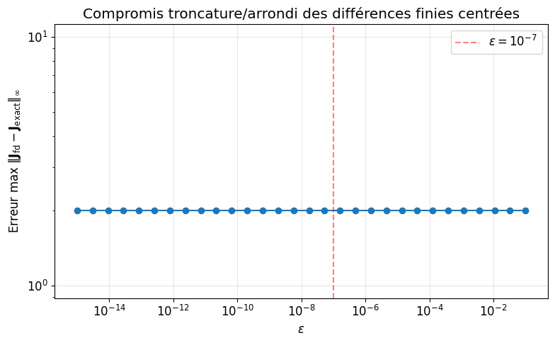
Récapitulatif¶

Ce TP a relié la notation de Spivak au code JAX. Le tableau suivant résume les correspondances.

À retenir:

1. La dérivée totale est une application linéaire, pas une matrice. La matrice jacobienne la représente.

2. Les dérivées partielles sont des restrictions: $\frac{\partial f_i}{\partial x_j} = \pi_i \circ Df(\mathbf{a}) \circ \iota_j$.

3. La règle de la chaîne est une composition d’applications linéaires. Pour le VJP, l’ordre de composition s’inverse.

4. Le VJP est le produit vecteur-jacobienne: $\mathbf{u}^\top \mathbf{J}_f(\mathbf{a})$.

5. Pour $f: \mathbb{R}^n \to \mathbb{R}^1$ (perte scalaire), un seul VJP donne le gradient complet, contre $n$ JVP. C’est le mode arrière (rétropropagation).

Pour aller plus loin: Chapitre 7: Réseaux de neurones, sections « Règles VJP » et « Implémentation minimale ».