Dynamics and State-Space Models

Models for Decision Making¶

“The sciences do not try to explain, they hardly even try to interpret, they mainly make models. By a model is meant a mathematical construct which, with the addition of certain verbal interpretations, describes observed phenomena. The justification of such a mathematical construct is solely and precisely that it is expected to work.” — John von Neumann

The word model means different things depending on who you ask.

In machine learning, it typically refers to a parameterized function (often a neural network) fit to data. When we say “we trained a model,” we usually mean adjusting parameters so it makes good predictions. This is a narrow view.

In control, operations research, or structural economics, a model refers more broadly to a formal specification of a decision problem. It includes how a system evolves over time, what parts of the world we choose to represent, what decisions are available, what can be observed or measured, and how outcomes are evaluated. It also encodes assumptions about time (discrete or continuous, finite or infinite horizon), uncertainty, and information structure.

To clarify terminology, we use the term decision-making model to refer to this broader object: one that includes system dynamics, state, control, observations, objectives, time structure, and information assumptions. In this sense, the model defines the structure of the decision problem. It is the formal scaffold on which we build optimization or learning procedures.

Depending on the setting, we may ask different things from a decision-making model. Sometimes we want a model that supports counterfactual reasoning or policy evaluation, and are willing to bake in more assumptions to get there. Other times, we just need a model that supports prediction or simulation, even if it remains agnostic about internal mechanisms.

This mirrors a distinction in econometrics between structural and reduced-form approaches. Structural models aim to capture the underlying process that generates behavior, enabling reasoning about what would happen under alternative policies or conditions. Reduced-form models, by contrast, focus on capturing statistical regularities (often to estimate causal effects) without necessarily modeling the mechanisms that generate them. Both are forms of modeling, just with different goals. The same applies in control and RL: some models are built to support simulation and optimization, while others serve more diagnostic or predictive roles, with fewer assumptions about how the system works internally.

This chapter focuses on the modeling side. What kinds of models do we need to support decision-making from data? What are their assumptions? What do they let us express or ignore? And how do they shape what learning and optimization can even mean?

Modeling, Realism, and Control¶

Realism is only one way to assess a model. When the purpose of modeling is to support control or decision making, accuracy in reproducing every detail of the system is not always necessary. What matters more is whether the model leads to decisions that perform well when applied in practice. A model may simplify the physics, ignore some variables, or group complex interactions into a disturbance term. As long as it retains the core feedback structure relevant to the control task, it can still be effective.

In some cases, high-fidelity models can be counterproductive. Their complexity makes them harder to understand, slower to simulate, and more difficult to tune. Worse, they may include uncertain parameters that do not affect the control decisions but still influence the outcome of optimization. The resulting decisions can become fragile or overfitted to details that are not stable across different operating conditions.

A useful model for control is one that focuses on the variables, dynamics, and constraints that shape the decisions to be made. It should capture the key trade-offs without trying to account for every effect. In traditional control design, this principle appears through model simplification: engineers reduce the system to a manageable form, then use feedback to absorb remaining uncertainty. Reinforcement learning adopts a similar mindset, though often implicitly. It allows for model error and evaluates success based on the quality of the policy when deployed, rather than on the accuracy of the model itself.

Example: A simple model that supports better decisions¶

Researchers at the U.S. National Renewable Energy Laboratory investigated how to reduce cooling costs in a typical home in Austin, Texas Cole et al., 2014. They had access to a detailed EnergyPlus simulation of the building, which included thousands of internal variables: layered wall models, HVAC cycling behavior, occupancy schedules, and detailed weather inputs.

Although this simulator could closely reproduce indoor temperatures, it was too slow and too complex to use as a planning tool. Instead, the researchers constructed a much simpler model using just two parameters: an effective thermal resistance $R$ and an effective thermal capacitance $C$. Treating the building as a single thermal mass, the indoor temperature $T$ evolves according to

where $T_{\text{out}}$ is the outdoor temperature and $Q_{\text{cool}}$ is the cooling power applied by the air conditioner. The first term on the right captures heat leaking in through the walls; the second captures heat removed by the cooling system. This is a first-order linear ODE, one of the simplest dynamics models possible.

This reduced model did not capture short-term temperature fluctuations and could be off by as much as two degrees on hot afternoons. Despite these inaccuracies, it proved useful for testing different cooling strategies. One such strategy involved cooling the house early in the morning when electricity prices were low, letting the temperature rise slowly during the expensive late-afternoon period, and resuming cooling only in the evening. When this strategy was simulated in the full EnergyPlus model, it reduced peak compressor power by approximately 70 percent and lowered total cooling cost by about 60 percent compared to a standard thermostat schedule.

The reason this worked is that the simple model captured the most important structural feature of the system: the thermal mass of the building (encoded in $C$) acts as a buffer that allows load shifting over time. The time constant $\tau = RC$ determines how quickly the indoor temperature responds to changes. That single number was enough to discover a control strategy that exploited this property. The many other effects present in the full simulation did not change the main conclusions and could be treated as part of the background variability.

This example shows that a model can be inaccurate in detail but still highly effective in guiding decisions. For control, what matters is not whether the model matches reality in every respect, but whether it helps identify actions that perform well under real-world conditions. We will return to this kind of thermal model, and its richer multi-zone extensions, once we have introduced the formal machinery.

Dynamics Models for Decision Making¶

The kind of model we need here is a dynamics model. It does not just describe correlations. It tells us how a system evolves in time and, for control purposes, how that evolution responds to inputs we choose.

A dynamics model earns its keep by answering counterfactuals of the form: given an initial condition and an input schedule, what trajectory should I expect? That ability to roll a trajectory forward under different candidate inputs is the backbone of planning, policy evaluation, and learning from interaction.

At this level, we can think of the model as a trajectory generator:

where $\mathbf{u}_t$ are controls we set, $\mathbf{d}_t$ are exogenous drivers we do not control (weather, inflow, demand), $\mathbf{x}_t$ are internal system variables, and $\mathbf{y}_t$ are observations. The split between $\mathbf{u}$ and $\mathbf{d}$ is practical: it separates what we can act on from what we must accommodate.

Two design pressures shape such models:

1. Responsiveness to inputs. The model must expose the levers that matter for the decision problem, even if everything underneath is approximate.

2. Memory management. To simulate step by step, we need a compact summary of the past that is sufficient to predict the next step once an input arrives. That summary is what we will call the state.

This brings us to a standard representation. Rather than carry the full history, we look for a variable $\mathbf{x}_t$ that captures “what matters so far” for predicting what comes next under a given input. With that variable in hand, the model advances in small increments and can be composed with estimators and controllers.

With this motivation in place, we can now introduce the formalism.

The State‑Space Perspective¶

Most dynamics models, whether derived from physics or learned from data, can be cast into state‑space form. The state $\mathbf{x}$ is the compact memory that summarizes the past for prediction and control. Inputs $\mathbf{u}$ perturb that state, exogenous drivers $\mathbf{d}$ push it around, and outputs $\mathbf{y}$ are what we can measure. The equations look the same whether time is treated in discrete steps or as a continuous variable.

Discrete versus continuous time¶

How we represent time is dictated by how we sense and actuate: digital controllers sample and apply inputs in steps; the underlying physics evolve continuously.

Time can be represented in two complementary ways, depending on how the system is sensed, actuated, or modelled.

In discrete time, we treat time as an integer counter, $t = 0, 1, 2, \dots$, advancing in fixed steps. This matches how digital systems operate: sensors are sampled periodically, decisions are made at regular intervals, and most logged data takes this form.

Continuous time treats time as a real variable, $t \in \mathbb{R}_{\ge 0}$. Many physical systems (mechanical, thermal, chemical) are most naturally expressed this way, using differential equations to describe how state changes.

The two views are interchangeable to some extent. A continuous-time model can be discretized through numerical integration, although this involves approximation. The degree of approximation depends on both the step size $\Delta t$ and the integration algorithm used. Conversely, a discrete-time policy can be extended to continuous time by holding inputs constant over time intervals (a zeroth-order hold), or by interpolating between values.

In physical systems, this hybrid setup is almost always present. Control software sends discrete commands to hardware (say, the output of a PID controller) which are then processed by a DAC (digital-to-analog converter) and applied to the plant through analog signals. The hardware might hold a voltage constant, ramp it, or apply some analog shaping. On the sensing side, continuous signals are sampled via ADCs before reaching a digital controller. So in practice, even systems governed by continuous dynamics end up interfacing with the digital world through discrete-time approximations.

This raises a natural question: if everything eventually gets discretized anyway, why not just model everything in discrete time from the start?

In many cases, we do. But continuous-time models can still be useful, sometimes even necessary. They often make physical assumptions more explicit, connect more naturally to domain knowledge (e.g. differential equations in mechanics or thermodynamics), and expose invariances or conserved quantities that get obscured by time discretization. They also make it easier to model systems at different time scales, or to reason about how behaviors change as resolution increases. So while implementation happens in discrete time, thinking in continuous time can clarify the structure of the model.

It is helpful to see how both representations look in mathematical form. The state-space equations are nearly identical with different notations depending on how time is represented.

Discrete time

Having defined state as the summary we carry forward, a step of prediction applies the chosen input and advances the state.

$\mathbf{x}_{t+1} = f_t(\mathbf{x}_t, \mathbf{u}_t), \qquad \mathbf{y}_t = h_t(\mathbf{x}_t, \mathbf{u}_t).$

Continuous time

$\dot{\mathbf{x}}(t) = f(\mathbf{x}(t), \mathbf{u}(t)), \qquad \mathbf{y}(t) = h(\mathbf{x}(t), \mathbf{u}(t)).$

The dot denotes a derivative with respect to real time; everything else (state, control, observation) remains the same.

When the functions $f$ and $h$ are linear we obtain

Linearity is not a belief about the world, it is a modeling choice that trades fidelity for transparency and speed.

$\dot{\mathbf{x}} = A\mathbf{x} + B\mathbf{u}, \qquad \mathbf{y} = C\mathbf{x} + D\mathbf{u}.$

The matrices $A, B, C, D$ may vary with $t$. Readers with an ML background will recognise the parallel with recurrent neural networks: the state is the hidden vector, the control the input, and the output the read‑out layer.

Classical control often moves to the frequency domain, using Laplace and Z‑transforms to turn differential and difference equations into algebraic ones. That is invaluable for stability analysis of linear time‑invariant systems, but the time‑domain state‑space view is more flexible for learning and simulation, so we will keep our primary focus there.

Examples of Deterministic Dynamics: HVAC Control¶

Consider a building in Montréal in the middle of February. Outside it is -20°C, and a thermostat tries to keep the interior comfortable. When the indoor temperature drops below your setpoint, the heating system kicks in. That system (a small building, a heater, the surrounding weather) can be modeled mathematically.

We start with a very simple approximation: treat the entire room as a single “thermal mass,” like a big air-filled box that heats up or cools down depending on how much heat flows in or out.

Let $\mathbf{x}(t)$ be the indoor air temperature at time $t$, and $\mathbf{u}(t)$ be the heating power supplied by the HVAC system. The outside air temperature, denoted $\mathbf{d}(t)$, affects the system too, acting as a known disturbance. Then the rate of change of indoor temperature is:

Here:

• $R$ is a thermal resistance: how well the walls insulate.

• $C$ is a thermal capacitance: how much energy it takes to heat the air.

This is a continuous-time linear system, and we can write it in standard state-space form:

with:

• $\mathbf{x}(t)$: indoor air temperature (the state)

• $\mathbf{u}(t)$: heater input (the control)

• $\mathbf{d}(t)$: outdoor temperature (disturbance)

• $\mathbf{y}(t)$: observed indoor temperature (output)

• $\mathbf{A} = -\frac{1}{RC}$

• $\mathbf{B} = \frac{1}{C}$

• $\mathbf{E} = \frac{1}{RC}$

• $\mathbf{C} = 1$

This model is simple, but too simplistic. It ignores the fact that the walls themselves store heat and release it slowly. This kind of delay is called thermal inertia: even if you turn the heater off, the walls might continue to warm the room for a while.

Before reading on, try to guess: if we want to capture the fact that walls store heat, what new variable should we add to the state? How would heat flow between the air and this new variable?

To capture this effect, we need to expand our state to include the wall temperature. We now model two coupled thermal masses: one for the air, and one for the wall. Heat can flow from the heater into the air, from the air into the wall, and from the wall out to the environment. This gives a more realistic description of how heat moves through a building envelope.

We write down an energy balance for each mass:

• For the air:

• For the wall:

Each term on the right-hand side corresponds to a flow of heat: the air gains heat from the wall and the heater, and the wall exchanges heat with both the air and the outside.

Now define the state vector:

Dividing both equations by their respective capacitances and rearranging terms, we arrive at the coupled system:

with:

Each entry in $\mathbf{A}$ has a physical interpretation:

• $A_{11}$: heat loss from the air to the wall

• $A_{12}$: heat gain by the air from the wall

• $A_{21}$: heat gain by the wall from the air

• $A_{22}$: net loss from the wall to both the air and the outside

The temperatures are now dynamically coupled: any change in one affects the other. The wall acts as a buffer that absorbs and releases heat over time.

This is still a linear system, just with a 2D state. But already it behaves differently. The walls absorb and release heat, smoothing out fluctuations and slowing down the response of the system.

As we add more rooms, walls, or building elements, the system grows. Each new temperature adds a new state. The equations still have the same structure, and their sparsity follows the building layout. Nodes represent temperatures; edges encode how heat flows between them.

Control Abstraction Levels¶

This network of states is what we control. What we mean by “control input” $\mathbf{u}(t)$ depends on both what we want to achieve and what we can implement in practice.

The most direct interpretation is to let $\mathbf{u}(t)$ represent the actual heating power delivered to the system, measured in watts. This makes sense when modeling from physical principles or simulating a system with fine-grained actuation.

In many real buildings, however, thermostats do not issue power commands. They activate a relay, turning the heater on or off based on whether the measured temperature crosses a setpoint. Some systems allow for modulated control—such as varying fan speed or partially opening a valve—but those details are often hidden behind firmware or closed controllers.

A common implementation involves a PID control loop that compares the measured temperature to a setpoint and adjusts the control signal accordingly. While the actual logic might be simple, the resulting behavior appears smoothed or delayed from the perspective of the building.

Depending on the abstraction level, we might:

• Treat $\mathbf{u}(t)$ as continuous power input, if designing the full control logic.

• Use it as a setpoint input, assuming a lower-level controller handles the rest.

• Or reduce it to a binary signal—heater on or off—when working with logged behavior from a smart thermostat.

Each perspective shapes the kind of model we build and the kind of control problem we pose. If we are designing a controller from scratch, it may be worth modeling the full closed-loop dynamics. If the goal is to tune setpoints or learn policies from data, a coarser abstraction may be both sufficient and more robust.

Advantages of Physics-Based Models¶

At this point, one might ask: why build this kind of physics-based model at all? If we can log indoor temperatures, thermostat actions, and weather data, we could instead learn a model directly from data. A neural ODE, for example, would let us define a parameterized function:

with both $f_{\boldsymbol{\theta}}$ and $g_{\boldsymbol{\theta}}$ learned from data. The internal state $\mathbf{z}(t)$ is not tied to any physical quantity. It just needs to be expressive enough to explain the observations.

That flexibility can be useful, particularly when a large dataset is already available. But in building control and energy modeling, the constraints are usually different.

Often, the engineer or consultant on site is working under tight time and information budgets. A floor plan might be available, along with some basic specs on insulation or window types, and a few days of logged sensor data. The task might be to simulate load under different weather scenarios, tune a controller, or just help understand why a room is slow to heat up. The model has to be built quickly, adapted easily, and remain understandable to others working on the same system.

In that context, RC models are often the default choice: not because they are inherently better, but because they fit the workflow.

The parameters of an RC model correspond to quantities one can reason about: thermal resistance, capacitance, heat transfer between zones. Values can be cross-checked against architectural plans or adjusted manually when something does not line up. It is straightforward to tell which wall or zone is contributing to slow recovery times.

RC models can often be calibrated from short data traces, even when not all state variables are directly observable. The structure already imposes constraints: heat flows from hot to cold, dynamics are passive, responses are smooth. Those properties help narrow the space of valid parameter settings. A neural ODE, in contrast, typically needs more data to settle into stable and plausible dynamics, especially if no additional constraints are enforced during training.

Once built, an RC model is straightforward to modify. If a window is replaced, or a wall gets insulated, only a few numbers need updating. The model is easy to pass along to another engineer or embed in a larger simulation. A model like

is linear and low-dimensional. Simulating it is cheap, even if you do it many times. That may not matter now, but it will matter later, when we want to optimize over trajectories or learn from them.

RC models are not always sufficient. They simplify or ignore many effects: solar gains, occupancy, nonlinearities, humidity, equipment switching behavior. If those effects are significant, and you have enough data, a black-box model (neural ODE or otherwise) might achieve lower prediction error. In practice, it is common to combine the two: use the RC structure as a backbone, and learn a residual model to correct for unmodeled dynamics.

Questions to consider: What changes if the building has multiple zones with different setpoints? How would you model a heat pump that can both heat and cool? If the thermostat only records on/off events, can you still identify the thermal parameters?

Simulating the 1R1C Model¶

Given a dynamics model, the next step is often simulation: computing a trajectory from an initial condition under a given input schedule. For a continuous-time ODE like the 1R1C model, this means numerical integration.

The simplest approach is the forward Euler method: approximate the derivative by a finite difference and step forward in time.

import numpy as np
import matplotlib.pyplot as plt

# 1R1C building model parameters
R = 2.0    # thermal resistance (°C/kW)
C = 10.0   # thermal capacitance (kWh/°C)
tau = R * C  # time constant (hours)

# Simulation parameters
dt = 0.1   # time step (hours)
T = 24     # total simulation time (hours)
n_steps = int(T / dt)

# Initial condition and inputs
T_in = np.zeros(n_steps + 1)
T_in[0] = 18.0  # initial indoor temperature (°C)

# Outdoor temperature: sinusoidal with daily cycle
t = np.linspace(0, T, n_steps + 1)
T_out = -10 + 5 * np.sin(2 * np.pi * t / 24 - np.pi/2)  # cold winter day

# Heating power: constant 2 kW
Q_heat = 2.0 * np.ones(n_steps)

# Forward Euler integration
for k in range(n_steps):
    dT_dt = (1/(R*C)) * (T_out[k] - T_in[k]) + (1/C) * Q_heat[k]
    T_in[k+1] = T_in[k] + dt * dT_dt

# Plot results
fig, (ax1, ax2) = plt.subplots(2, 1, figsize=(8, 5), sharex=True)
ax1.plot(t, T_in, label='Indoor', linewidth=2)
ax1.plot(t, T_out, '--', label='Outdoor', linewidth=1.5)
ax1.set_ylabel('Temperature (°C)')
ax1.legend()
ax1.set_title(f'1R1C Building Model (τ = {tau:.0f} hours)')
ax1.grid(True, alpha=0.3)

ax2.step(t[:-1], Q_heat, where='post', linewidth=2)
ax2.set_xlabel('Time (hours)')
ax2.set_ylabel('Heating power (kW)')
ax2.set_ylim(0, 3)
ax2.grid(True, alpha=0.3)
plt.tight_layout()
plt.show()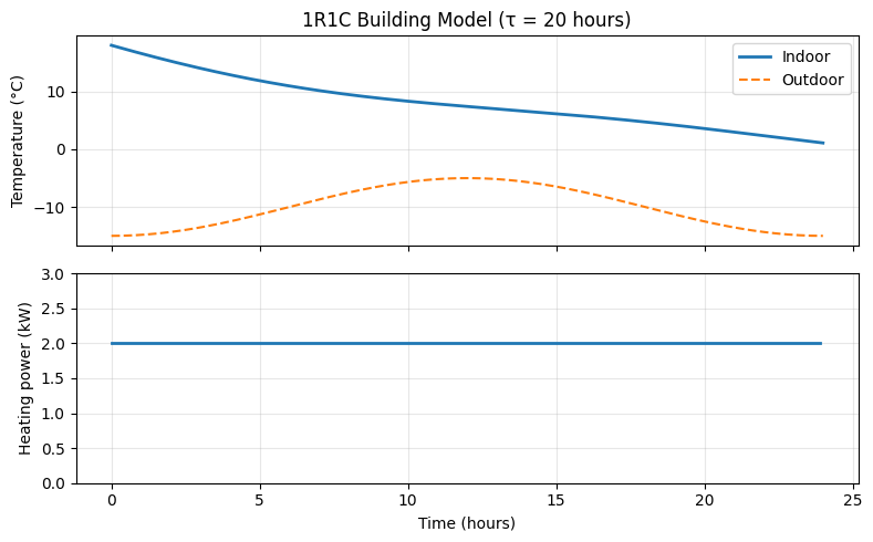

The time constant $\tau = RC = 20$ hours means the building responds slowly to changes. Even with constant heating, it takes several hours for the indoor temperature to stabilize. This slow response is exactly what enables load-shifting strategies: pre-heat when electricity is cheap, and coast through expensive periods.

From Deterministic to Stochastic¶

The models considered so far were deterministic: given an initial state and input sequence, the system evolves in a fixed, predictable way. But real systems rarely behave so neatly. Sensors are noisy. Parameters drift. The world changes in ways we cannot fully model.

To account for this uncertainty, we move from deterministic dynamics to stochastic models. There are two equivalent but conceptually distinct ways to do this.

Function plus Noise¶

The most direct extension adds a noise term to the dynamics:

If the noise is additive and Gaussian, we recover the standard linear-Gaussian setup used in Kalman filtering:

We are not restricted to Gaussian or additive noise. For instance, if the noise distribution is non-Gaussian:

then $\mathbf{x}_{t+1}$ inherits those properties. This is known as a convolution model: the next-state distribution is a shifted version of the noise distribution, centered around the deterministic prediction. More formally, this is a special case of a pushforward measure: the randomness from $\mathbf{w}_t$ is “pushed forward” through the function $f$ to yield a distribution over outcomes.

Or the noise might enter multiplicatively:

where $\Gamma$ is a matrix that modulates the effect of the noise, potentially depending on state and control. If $\Gamma$ is invertible, we can even write down an explicit density via a change-of-variables:

This kind of structured noise is common in practice, for example, when disturbances are amplified at certain operating points.

The function-plus-noise view is natural when we have a physical or simulator-based model and want to account for uncertainty around it. It is constructive: we know how the system evolves and how the randomness enters. This means we can track the source of variability along a trajectory, which is particularly useful for techniques like reparameterization or infinitesimal perturbation analysis (IPA). These methods rely on being able to differentiate through the noise injection mechanism, something that is much easier when the noise is explicit and structured.

Consider: if all we can do is sample next states from a simulator—without knowing the internal noise source—can we still write down a dynamics model? What form would it take?

Transition Kernel¶

The second perspective skips over the internal noise and defines the system directly in terms of the probability distribution over next states:

This transition kernel encodes all the uncertainty in the evolution of the system, without reference to any underlying noise source or functional form.

This view is strictly more general: it includes the function-plus-noise case as a special instance. If we do know the function $f$ and the noise distribution $p_{\mathbf{w}}$ from the generative model, then the transition kernel is obtained by “pushing” the randomness through the function:

This may look abstract, but it is just marginalization: for each possible noise value $\mathbf{w}$, we compute the resulting next state, and then average over all possible $\mathbf{w}$, weighted by how likely each one is.

If the noise were discrete, this becomes a sum:

This abstraction is especially useful when we do not know (or do not care about) the underlying function or noise distribution. All we need is the ability to sample transitions or estimate their likelihoods. This is the default formulation in reinforcement learning, econometrics, and other settings focused on behavior rather than mechanism.

To summarize: we have two views of stochastic dynamics. The function-plus-noise view is constructive; it tells us exactly how randomness enters and allows differentiation through the noise. The transition kernel view is more abstract but more general; it only requires that we can sample or evaluate likelihoods. Both describe the same object; the choice depends on what we know and what we need to compute.

Continuous-Time Analogue¶

In continuous time, the stochastic dynamics of a system are often described using a stochastic differential equation (SDE):

where $\mathbf{W}_t$ is Brownian motion. The first term, called the drift, describes the average motion of the system. The second, scaled by $\sigma$, models how random fluctuations (diffusion) enter over time. Just like in discrete time, this is a function + noise model: the state evolves through a deterministic path perturbed by stochastic input.

This generative view again induces a probability distribution over future states. At any future time $t + \Delta t$, the system does not land at a single state but is described by a distribution that depends on the initial condition and the noise along the way.

Mathematically, this distribution evolves according to the Fokker–Planck equation, a partial differential equation that governs how probability density “flows” through time. It plays the same role here as the transition kernel did in discrete time: describing how likely the system is to be in any given state, without referring to the noise directly.

While the mathematical generalization is clean, working with continuous-time stochastic models can be more challenging. Simulating sample paths is often straightforward (eg. nowadays diffusion models in generative AI), but writing down or computing the exact transition distribution usually is not. For this reason, many practical methods still rely on discrete-time approximations, even when the underlying system is continuous.

Example: Managing a Québec Hydroelectric Reservoir¶

On the James Bay plateau, 1 400 km north of Montréal, the Robert-Bourassa reservoir stores roughly 62 km³ of water, more than the volume of Lake Ontario above its minimum operating level. Sixteen giant turbines sit 140 m below the surface, converting that stored head into 5.6 GW of electricity, about a fifth of Hydro-Québec’s total capacity. A steady share of that output feeds Québec’s aluminium smelters, which depend on stable, uninterrupted power.

Water managers face competing objectives:

• Flood safety. Sudden snowmelt or storms can overfill the basin, forcing emergency spillways to open. These events are spectacular, but carry real downstream risk and economic cost.

• Energy reliability. If the level falls too low, turbines sit idle and contracts go unmet. Voltage dips at the smelters are measured in lost millions.

A basic deterministic model for the mass balance of the reservoir is straightforward bookkeeping:

where $\mathbf{x}_t$ is the current reservoir level, $\mathbf{u}_t$ is the controlled outflow through turbines, and $\mathbf{r}_t$ is the natural inflow from rainfall and upstream runoff.

But inflow is variable, and its statistical structure matters. Two hydrological regimes dominate:

• In spring, melting snow over days can produce a long-tailed inflow distribution, often modeled as log-normal or Gamma.

• In summer, convective storms yield a skewed mixture: a point mass at zero (no rain), and a thin but heavy tail capturing sudden bursts.

This motivates a simple stochastic extension:

Here the physics is fixed, and all uncertainty sits in the inflow term $\mathbf{w}_t$. Rather than fitting a full transition model from $(\mathbf{x}_t, \mathbf{u}_t)$ to $\mathbf{x}_{t+1}$, we can isolate the inflow by rearranging the mass balance:

This gives a direct estimate of the realized inflow at each timestep. From there, the problem becomes one of density estimation: fit a probabilistic model to the residuals $\hat{\mathbf{w}}_t$. In spring, this might be a log-normal distribution. In summer, a two-part mixture: a point mass at zero, and an exponential tail. These distributions can be estimated by maximum likelihood, or adjusted using additional features (covariates) such as upstream snowpack or forecasted temperature.

This setup has practical benefits. Fixing the physical part of the model (how levels respond to inflow and outflow) helps focus the statistical modeling effort. Rather than fitting a full system model, we only need to estimate the variability in inflows. This reduces the number of degrees of freedom and makes the estimation problem easier to interpret. It also avoids conflating uncertainty in inflow with uncertainty in the response of the system.

To get a sense of scale: the Robert-Bourassa reservoir has a usable storage range of roughly 20 km³. Weekly inflows during spring freshet might average 1.5 km³ with a standard deviation of 0.4 km³. A manager planning turbine releases might simulate 1000 inflow scenarios over a 52-week horizon to estimate the probability of overflow or shortage under different release policies. Each scenario is just a draw from the fitted inflow distribution, pushed through the deterministic mass balance.

Compare this to a more generic approach, such as linear regression:

This is straightforward to fit, but offers no guarantee that the result behaves sensibly. The model might violate conservation of mass, or compensate for inflow variation by adjusting coefficients $a$ and $b$. This can lead to misleading conclusions, especially when extrapolating beyond the training data.

Questions to consider: How would you incorporate weather forecasts into the inflow model? What if the reservoir is part of a cascade, where releases from one dam become inflows to the next? How would you handle the fact that inflow distributions differ by season?

Partial Observability¶

So far, we have assumed that the full system state $\mathbf{x}_t$ is available. But in most real-world settings, only a partial or noisy observation is accessible. Sensors have limited coverage, measurements come with noise, and some variables are not observable at all.

To model this, we introduce an observation equation alongside the system dynamics:

The state $\mathbf{x}_t$ evolves under control inputs $\mathbf{u}_t$ and process noise $\mathbf{w}_t$, but we do not observe $\mathbf{x}_t$ directly. Instead, we observe $\mathbf{y}_t$, which depends on $\mathbf{x}_t$ through some possibly nonlinear, noisy function $h_t$. The noise $\mathbf{v}_t$ captures measurement uncertainty.

This setup defines a partially observed system. Even if the underlying dynamics are known, we still face uncertainty due to limited visibility into the true state. The controller or estimator must rely on the observations $\mathbf{y}_{0\:t}$ to make sense of the hidden trajectory.

In the deterministic case, if the output map $h_t$ is full-rank and invertible, we may be able to reconstruct the state directly from the output: no filtering required. But once noise is introduced, that invertibility becomes more subtle: even if $h_t$ is bijective, the presence of $\mathbf{v}_t$ prevents us from recovering $\mathbf{x}_t$ exactly. In this case, we must shift from inversion to estimation, often via probabilistic inference.

In the linear-Gaussian case, the model simplifies to:

This is the classical state-space model used in signal processing and control. The model is fully specified by the system matrices and the covariances $Q$ and $R$. The state is no longer known, but under these assumptions it can be estimated recursively using the Kalman filter, which maintains a Gaussian belief over $\mathbf{x}_t$.

Even when the model is nonlinear or non-Gaussian, the structure remains the same: a dynamic state evolves, and a separate observation process links it to the data we see. Many modern estimation techniques, including extended and unscented Kalman filters, particle filters, and learned neural estimators, build on this core structure.

Observation Kernel View¶

Just as we moved from function-based dynamics to transition kernels, we can abstract away the noise source and define the observation distribution directly:

This kernel summarizes what the sensors tell us about the hidden state. If we know the generative model—say, that $\mathbf{y}_t = h_t(\mathbf{x}_t) + \mathbf{v}_t$ with known $p_{\mathbf{v}}$—then this kernel is induced by marginalizing out $\mathbf{v}_t$:

But we do not have to start from the generative form. In practice, we might define or learn $p(\mathbf{y}_t \mid \mathbf{x}_t)$ directly, especially when dealing with black-box sensors, perception models, or abstract measurement processes.

Example – Stabilizing a Telescope’s Vision with Adaptive Optics¶

On Earth, even the largest telescopes cannot see perfectly. As starlight travels through the atmosphere, tiny air pockets with different temperatures bend the light in slightly different directions. The result is a distorted image: instead of a sharp point, a star looks like a flickering blob. The distortion happens fast, on the order of milliseconds, and changes continuously as wind moves the turbulent layers overhead.

Adaptive optics (AO) systems cancel out these distortions in real time by measuring how the incoming wavefront of light is distorted and using a flexible mirror to apply a counter-distortion that straightens it back out. The difficulty is that the wavefront cannot be observed directly. The sensor provides only noisy measurements of its slopes (the angles of tilt at various points), and the controller must act fast, before the atmosphere changes again.

To design a controller here, we need a model of how the distortions evolve. And that means building a decision-making model: one that includes uncertainty, partial observability, and fast feedback.

The main object to track is the distortion of the incoming wavefront. This phase field $\phi(\mathbf{r}, t)$ cannot be observed directly, but we can represent it approximately using a finite basis (e.g., Fourier or Zernike). The coefficients of this expansion form our internal state:

A typical system might use $n = 100$ to 500 Zernike modes, sampled at 1–2 kHz. The state dimension is modest, but the control loop must complete in under a millisecond to keep up with the atmosphere.

The atmosphere evolves in time. A simple but effective model assumes the turbulence is “frozen” and just blown across the telescope by the wind. That gives us a discrete-time linear model:

where $\mathbf{A}$ shifts the distortion pattern in space, and $\mathbf{w}_t$ is a small random change from evolving turbulence. This noise is not arbitrary: its statistics follow a power law derived from Kolmogorov’s turbulence model. In particular, higher spatial frequencies (small-scale wiggles) have less energy than low ones. This allows us to build a prior on how likely different distortions are.

The full wavefront is not directly observable. Instead, we use a wavefront sensor: a camera that captures how the light bends. What it actually measures are local slopes, the gradients of the wavefront, not the wavefront itself. So our observation model is:

where $\mathbf{C}$ is a known matrix that maps wavefront distortion to measurable slope angles, and $\boldsymbol{\varepsilon}_t$ is measurement noise (e.g., due to photon limits).

The control objective is to flatten the wavefront using a deformable mirror. The mirror can apply a small counter-distortion $\mathbf{u}_t$ that subtracts from the atmospheric one:

The goal is to choose $\mathbf{u}_t$ to minimize the residual distortion by making the light flat again.

Without a model, we would just react to the current noisy measurements. With a model, we can predict how the wavefront will evolve, filter out noise, and act preemptively. This is essential in AO, where decisions must be made every millisecond. Kalman filters are often used to track the hidden state $\mathbf{x}_t$, combining model predictions with noisy measurements, and linear-quadratic regulators (LQR) or other optimal controllers use those estimates to choose the best correction.

Adaptive optics is a rare case where continuous-time modeling also plays a role. The true evolution of the turbulence is continuous, and we can model it using a stochastic differential equation (SDE):

where $\mathbf{W}(t)$ is Brownian motion and the matrix $\mathbf{G}$ encodes the Kolmogorov spectrum. Discretizing this equation gives us the $\mathbf{A}$ and $\mathbf{Q}$ matrices for the discrete-time model above.

Questions to consider: What happens if the wind speed changes suddenly—does the frozen-flow assumption break down? How might you adapt the model online as conditions change? If the guide star is faint and photon noise dominates, how does that affect the observation model?

Programs as Models¶

Consider again the HVAC example from earlier in this chapter. We wrote down a simple RC model: $\dot{T} = \frac{1}{RC}(T_{\text{out}} - T) + \frac{1}{C}Q$. Given the parameters $R$ and $C$, we can compute the temperature at any future time by solving the differential equation. We have direct access to the dynamics function itself.

Now imagine instead that we are given only a software tool—say, EnergyPlus—that simulates the building. We can feed it an initial temperature and a schedule of heating commands, press “run,” and observe the resulting temperature trajectory. But we cannot inspect the internal equations. We cannot take a derivative of the output with respect to a parameter. We can only query the simulator as a black box.

This distinction matters for control. Many algorithms assume we can evaluate $f(\mathbf{x}, \mathbf{u})$ at arbitrary points, or even differentiate through it. When the model is a program rather than an equation, these operations are not always available, and we must adapt our methods accordingly.

Up to this point, we have described models using systems of equations—either differential or difference equations—that express how a system evolves over time. These analytical models define the transition structure explicitly. For instance, in discrete time, the evolution of the state is governed by a known function:

Given access to $f$, we can construct trajectories, analyze system behavior, and design control policies. The important feature here is not that the model evolves one step at a time, but that we are given the local dynamics function $f$ itself.

In contrast, simulation-based models do not expose $f$ directly. Instead, they define a procedure—implemented in code—that takes an initial state and input sequence and returns the resulting trajectory:

Here, $\mathcal{S}$ represents the full simulator. Internally, it may apply numerical integration, scheduling logic, branching rules, or other computations. But these details are encapsulated. From the outside, we can only query the simulator by running it.

This distinction is subtle but important. Both types of models can generate trajectories. What matters is the interface: analytical models provide direct access to $f$; simulation models do not. They offer a trajectory-generation interface, but hide the internal structure that produces it.

Before reading on, think about which category the examples from earlier in this chapter fall into. Is the RC thermal model analytical or simulation-based? What about the reservoir model? The adaptive optics system?

Case Study: Robotics with MuJoCo¶

MuJoCo simulates the dynamics of articulated rigid bodies under contact constraints. The equations it solves include:

$M(\mathbf{q})\ddot{\mathbf{q}} + C(\mathbf{q}, \dot{\mathbf{q}}) = \boldsymbol{\tau} + J^\top \boldsymbol{\lambda}$

$\phi(\mathbf{q}) = 0, \quad \boldsymbol{\lambda} \geq 0, \quad \boldsymbol{\lambda}^\top \phi = 0$

Here $\mathbf{q}$ are joint positions, $M$ is the mass matrix, and $\boldsymbol{\lambda}$ are contact forces enforcing non-penetration. But these physical equations are part of a larger simulator that also includes collision detection, contact force models, sensor and actuator emulation, and visual rendering.

The full behavior of a robot interacting with its environment emerges only when the simulator is executed. While the underlying physics are well-understood, the complexity of contact dynamics, collision detection, and sensor modeling makes it impractical to expose the local dynamics function $f$ directly.

Questions to consider: If you can only query MuJoCo as a black box, how would you estimate the gradient of a cost function with respect to the control inputs? What changes if you have access to the simulator’s source code?

Systems with Discrete Events¶

Many simulation models arise when a system’s dynamics are driven not by time-continuous evolution, but by the occurrence of events. These discrete-event systems (DES) change state only at specific, often asynchronous points in time. Between events, the state remains fixed.

A discrete-event system can be described by:

• a set of discrete states $\mathcal{X}$,

• a set of events $\mathcal{E}$,

• a transition function $f: \mathcal{X} \times \mathcal{E} \rightarrow \mathcal{X}$,

• and a time-advance function $t_a: \mathcal{X} \rightarrow \mathbb{R}_{\geq 0}$.

At each point, the system checks which events are enabled and advances to the next scheduled one.

Consider a software-defined networking (SDN) controller managing traffic routing in a data center. The system must make real-time decisions about packet forwarding paths based on network conditions and service requirements.

The discrete states $\mathcal{X}$ represent the current network configuration: active routing tables, link utilization levels, and quality-of-service priority queues at each switch.

The events $\mathcal{E}$ include new flow requests arriving (video streaming, database queries, file transfers), link failures or congestion threshold violations, flow completion notifications, load balancing triggers when servers exceed capacity, and network policy updates from administrators.

The transition function $f$ captures how routing decisions change the network state. When a high-priority video conference flow arrives while a link is congested, the controller might transition to a new state where low-priority background traffic is rerouted through alternative paths.

The time-advance function $t_a$ determines when the next routing decision occurs. Flow arrivals follow traffic patterns (bursty during business hours), while link failures are rare but unpredictable events.

Between events, packets follow the established routing rules; the same forwarding tables remain active across all switches. The control problem here is to adapt routing decisions to discrete network events, balancing throughput, latency, and reliability constraints.

Questions to consider: How would you define a “state” for this system in a way that is Markovian? What information would you need to predict the next event time?

Hybrid Systems¶

Some systems evolve continuously most of the time but undergo discrete jumps in response to certain conditions. These hybrid systems are common in control applications.

The system consists of:

• a set of discrete modes $q \in \mathcal{Q}$,

• continuous dynamics in each mode: $\dot{\mathbf{x}} = f_q(\mathbf{x})$,

• guards that specify when transitions between modes occur,

• and reset maps that update the state during such transitions.

An HVAC system can be in one of several modes: heating, cooling, or off. The temperature evolves continuously according to physical laws, but when it crosses certain thresholds, the system switches modes:

if x < setpoint - delta:
    mode = "heating"
elif x > setpoint + delta:
    mode = "cooling"
else:
    mode = "off"

Within each mode, a different differential equation applies. This results in a piecewise-smooth trajectory with mode-dependent dynamics.

Case Study: Building Energy with EnergyPlus¶

EnergyPlus provides a detailed example of hybrid systems in building energy simulation. At its core are physical equations describing heat flows:

It also solves implicit equations representing HVAC component behavior:

But the actual simulator includes hundreds of thousands of lines of code handling interpolated weather data, occupancy schedules, equipment performance curves, and control logic implemented as finite-state machines.

The result is a program that emulates how a building behaves over time, given environmental inputs and schedules. The hybrid nature emerges from the interaction between continuous thermal dynamics and discrete control decisions made by thermostats, occupancy sensors, and HVAC equipment.

Questions to consider: How does EnergyPlus relate to the simple RC models we derived earlier? Could you use an RC model as a surrogate for optimization, then validate in EnergyPlus?

Agent-Based Models¶

Some simulation models do not describe systems via global state transitions, but instead simulate the behavior of many individual components or agents, each following local rules. These agent-based models (ABMs) are widely used in epidemiology, ecology, and social modeling.

Each agent maintains its own internal state and acts according to probabilistic or rule-based logic. The system’s behavior arises from the interactions among agents.

Consider a neighborhood where each household is an agent making energy consumption decisions based on real-time electricity pricing and thermal comfort preferences. Each household agent has internal state (current temperature, HVAC settings, comfort preferences, price sensitivity), local decision rules (MPC algorithms that optimize the trade-off between energy cost and thermal comfort), and unique characteristics (different utility functions, thermal mass, occupancy patterns).

The simulator might execute something like:

for household in neighborhood:
    # Each household solves its own MPC optimization
    current_price = utility.get_current_price()
    comfort_weight = household.comfort_preference
    
    # Optimize over prediction horizon
    optimal_setpoint = household.mpc_controller.optimize(
        current_temp=household.temperature,
        price_forecast=utility.price_forecast,
        comfort_weight=comfort_weight
    )
    
    household.set_hvac_setpoint(optimal_setpoint)
    
    # Update shared grid load
    neighborhood.total_demand += household.power_consumption

The macro-level demand patterns—peak shifting, load leveling, rebound effects—emerge from individual household optimization decisions. No single equation describes the neighborhood’s energy consumption; it arises from the collective behavior of autonomous agents each solving their own control problems.

Case Study: Traffic Simulation with SUMO¶

SUMO is an agent-based traffic simulator used in transportation research. Each vehicle is an agent with its own route, driving behavior, and decision-making logic. The Krauss car-following rule shows how individual vehicle agents behave:

def update_vehicle(v, v_leader, gap, dt):
    v_safe = v_leader + (gap - min_gap) / tau
    v_desired = min(v_max, v_safe)
    ε = random.uniform(0, 1)
    v_new = max(0, v_desired - ε * a_max * dt)
    x_new = x + v_new * dt
    return x_new, v_new

Beyond car-following, each vehicle agent also plans routes through the network based on travel time estimates, responds to traffic signals and road conditions, makes lane-changing decisions based on utility functions, and exhibits individual driving characteristics (aggressiveness, reaction time).

The emergent traffic patterns—congestion formation, traffic waves, bottlenecks—arise from the collective behavior of thousands of individual vehicle agents, each following local rules and making autonomous decisions.

Questions to consider: In an agent-based model, what plays the role of the “state”? Is it the collection of all agent states? How would you define a policy that controls traffic signals based on this high-dimensional state?

To summarize the taxonomy so far: we have moved from analytical models (where the dynamics function $f$ is given explicitly) to simulation-based models (where we can only query trajectories). Within simulation-based models, we distinguished three patterns: discrete-event systems, where the state changes only at specific events; hybrid systems, where continuous dynamics interact with discrete mode switches; and agent-based models, where macro-level behavior emerges from local agent interactions.

This distinction will matter throughout the book. When we have access to the dynamics function $f$, we can use gradient-based trajectory optimization (Chapter 3) or derive closed-form solutions like the Riccati equation for LQR. When we only have simulator access, we must rely on sampling-based methods: Monte Carlo estimation, reinforcement learning, and derivative-free optimization. The model interface shapes the algorithms we can apply.

The following case study illustrates how these ideas combine in practice.

Case Study: Curbside Access at Montréal–Trudeau Airport¶

Afternoon traffic at Montréal–Trudeau airport regularly backs up along the two-lane ramp leading to the departures curb. As passenger volumes rebound, the mix of private drop-offs, taxis, and shuttles converging in a confined space produces frequent delays. When curb dwell times rise, especially around wide-body departures, queues can spill back onto the access road and interfere with other flows on the airport campus.

To manage the situation, the airport operator relies on a dense sensor network. Cameras and license plate readers track vehicle trajectories across virtual gates, generating a real-time stream of entry points, curb interactions, and exit times. According to public statements, AI-based forecasting solutions have been deployed to anticipate congestion and suggest alternative routing options for passengers and drivers. While no technical details have been disclosed, this is a typical instance of a traffic prediction and control problem that lends itself to agent-based modeling.

In such a model, each vehicle is treated as an individual agent with internal state:

where $x_t$ and $v_t$ denote longitudinal position and speed, and lane and intent capture higher-level behavioral traits. The simulation proceeds in discrete time. At each step, agents update their acceleration based on local traffic density (e.g., via a car-following model like IDM), evaluate potential lane changes (e.g., using a utility or incentive rule), and advance position accordingly.

The layout of the ramp—its geometry, merges, and constraints—is fixed. What changes are the traffic patterns and driver behaviors. These can be estimated from historical trajectories and updated as new data arrives. In a real-time setting, a filtering step adjusts the simulation so that its predicted flows remain consistent with current observations.

While the behavior of each individual agent is governed by program logic and heuristics—such as car-following rules, desired speeds, or gap acceptance—some parameters are identified offline from historical data, while others are estimated online. This adaptation helps the model track observed conditions. But even with such adjustments, not all effects are easily captured.

Construction activity, weather disturbances, and irregular flight scheduling can introduce sudden shifts in flow that lie outside the scope of the structural model. To account for these, one can overlay a data-driven correction on top of the simulation. Suppose the simulator produces a queue length forecast $q^{\text{sim}}_{t+h}$ over horizon $h$. A statistical model can be trained to predict the residual between this forecast and the observed outcome:

as a function of exogenous features $z_t$, such as weather, incident flags, or scheduled arrivals. The final forecast then becomes:

where $\phi$ is a learned mapping from external conditions to the expected correction. The result is a hybrid model: the simulation enforces physical structure and agent-level behavior, while the residual model compensates for aspects of the system that are harder to express analytically.

Questions to consider: What are the tradeoffs between using a purely data-driven model versus a simulation with residual correction? How would you decide how much structure to build into the simulation versus how much to learn from data?

Summary¶

This chapter introduced the modeling vocabulary we use throughout the book.

A dynamics model describes how a system evolves in response to inputs we control and disturbances we cannot. The state-space representation provides a common language: the state $\mathbf{x}$ is a compact summary of the past sufficient to predict the future given the current input. This representation works for both discrete-time systems (difference equations) and continuous-time systems (differential equations), and for both linear and nonlinear dynamics.

The transition from deterministic to stochastic models adds uncertainty. We saw two equivalent views: the function-plus-noise perspective, which is constructive and allows differentiation through the randomness, and the transition kernel perspective, which is more abstract but requires only the ability to sample or evaluate likelihoods. The choice depends on what we know about the system and what we need to compute.

Partial observability adds another layer: the state is hidden, and we only see noisy projections through an observation model. This structure—hidden state, stochastic dynamics, noisy observations—is the foundation for state estimation (Kalman filtering, particle filtering) and for decision-making under uncertainty.

Beyond analytical models, we also considered simulation-based models where the dynamics function is not exposed directly. Instead, a program takes an initial state and input sequence and returns the resulting trajectory. This includes discrete-event systems (where state changes only at specific events), hybrid systems (where continuous dynamics interact with discrete mode switches), and agent-based models (where macro-level behavior emerges from local agent interactions). These simulation-based approaches are common in robotics, building energy, and traffic modeling.

Throughout, we emphasized that models for control need not be accurate in every detail. What matters is whether they capture the structure relevant to the decisions being made. A simple two-parameter thermal model can guide effective load-shifting strategies; a physics-based reservoir model with fitted inflow distributions can support robust planning; a linear model of atmospheric turbulence can enable real-time wavefront correction. The model is a tool for decision-making, not an end in itself.

There is no universally correct way to model a system. The choice depends on what we know, what we can observe, what we care about, and what tools we have. In every case, modeling choices define the structure of the problem and the space of possible solutions. The next chapter turns to numerical trajectory optimization: how to compute optimal trajectories given a dynamics model.