Weighted Residual Methods for Functional Equations

The Bellman optimality equation $\Bellman v = v$, whose contraction property underlies the convergence of value iteration, is a functional equation: an equation where the unknown is an entire function rather than a finite-dimensional vector. When the state space is continuous or very large, we cannot represent the value function exactly on a computer. We must instead work with finite-dimensional approximations. This motivates weighted residual methods (also called minimum residual methods), a general framework for transforming infinite-dimensional problems into tractable finite-dimensional ones Chakraverty et al. (2019)Atkinson & Potra (1987).

A Motivating Example: Optimal Stopping with Continuous States¶

Before developing the general theory, consider a concrete example that illustrates the core challenge. An agent observes a state $s \in [0, 1]$ and must decide whether to stop (receive reward $s$ and end the episode) or continue (receive nothing, and the state redraws uniformly on $[0, 1]$). With discount factor $\gamma = 0.9$, the Bellman optimality equation is:

The first term is the immediate payoff from stopping; the second is the discounted expected continuation value. Since the continuation value $\bar{v} = \int_0^1 v^*(s') ds'$ is a constant (it doesn’t depend on the current state $s$), the optimal policy has a threshold structure: stop if $s \geq s^*$ for some threshold $s^*$, continue otherwise.

At the threshold, the agent is indifferent: $s^* = \gamma \bar{v}$. Computing $\bar{v}$ by integrating $v^*$:

Substituting $s^* = \gamma \bar{v}$ and solving gives the exact threshold and value.

Source

#  label: fig-optimal-stopping-exact
#  caption: The exact value function for the optimal stopping problem.

%config InlineBackend.figure_format = 'retina'
import numpy as np
import matplotlib.pyplot as plt

gamma = 0.9

# Solve for exact threshold
v_bar_exact = (1 - np.sqrt(1 - gamma**2)) / gamma**2
s_star_exact = gamma * v_bar_exact

print(f"Exact solution:")
print(f"  Threshold s* = {s_star_exact:.6f}")
print(f"  Continuation value v̄ = {v_bar_exact:.6f}")

# The exact value function
def v_exact(s):
    return np.where(s >= s_star_exact, s, gamma * v_bar_exact)

# Plot the exact value function
s_grid = np.linspace(0, 1, 200)
plt.figure(figsize=(8, 4))
plt.plot(s_grid, v_exact(s_grid), 'b-', linewidth=2, label='Exact $v^*(s)$')
plt.axvline(s_star_exact, color='r', linestyle='--', label=f'Threshold $s^* = {s_star_exact:.3f}$')
plt.xlabel('State $s$')
plt.ylabel('Value $v^*(s)$')
plt.legend()
plt.title('Optimal Stopping: Exact Value Function')
plt.grid(True, alpha=0.3)
plt.tight_layout()

Exact solution:
  Threshold s* = 0.626789
  Continuation value v̄ = 0.696432

The exact value function is piecewise linear: constant at $\gamma \bar{v}$ below the threshold, equal to $s$ above it. Now suppose we want to approximate $v^*$ using a polynomial basis with $n$ terms:

The residual at state $s$ measures how far our approximation is from satisfying the Bellman equation:

For a perfect solution, $R(s; \theta) = 0$ for all $s \in [0, 1]$. But a polynomial cannot exactly represent the kink at $s^*$. We must choose how to make the residual “small” across the state space.

Collocation picks $n$ points $\{s_1, \ldots, s_n\}$ and requires the residual to vanish exactly there:

Galerkin requires the residual to be orthogonal to each basis function:

Source

#  label: fig-collocation-comparison
#  caption: Polynomial collocation approximation with 5 Chebyshev nodes.

from scipy.integrate import quad

def chebyshev_nodes(n, a=0, b=1):
    """Chebyshev nodes on [a, b]."""
    k = np.arange(1, n + 1)
    nodes = 0.5 * (a + b) + 0.5 * (b - a) * np.cos((2*k - 1) * np.pi / (2*n))
    return np.sort(nodes)

def collocation_solve(n, gamma, max_iter=100, tol=1e-8):
    """Solve optimal stopping via polynomial collocation."""
    nodes = chebyshev_nodes(n)
    Phi = np.vander(nodes, n, increasing=True)
    
    theta = np.zeros(n)
    for iteration in range(max_iter):
        def v_approx(s):
            return sum(theta[j] * s**j for j in range(n))
        
        v_bar, _ = quad(v_approx, 0, 1)
        targets = np.maximum(nodes, gamma * v_bar)
        theta_new = np.linalg.solve(Phi, targets)
        
        if np.linalg.norm(theta_new - theta) < tol:
            return theta_new, iteration + 1
        theta = theta_new
    return theta, max_iter

# Solve with different numbers of basis functions
for n in [3, 5, 8]:
    theta, iters = collocation_solve(n, gamma)
    def v_approx(s, theta=theta, n=n):
        return sum(theta[j] * s**j for j in range(n))
    errors = [abs(v_approx(s) - v_exact(s)) for s in np.linspace(0, 1, 1000)]
    print(f"n = {n}: converged in {iters} iters, max error = {max(errors):.6f}")

# Plot comparison for n=5
n = 5
theta, _ = collocation_solve(n, gamma)
v_approx_5 = lambda s: sum(theta[j] * s**j for j in range(n))

plt.figure(figsize=(8, 4))
plt.plot(s_grid, v_exact(s_grid), 'b-', linewidth=2, label='Exact')
plt.plot(s_grid, [v_approx_5(s) for s in s_grid], 'r--', linewidth=2, label=f'Collocation ($n={n}$)')
plt.scatter(chebyshev_nodes(n), [v_approx_5(s) for s in chebyshev_nodes(n)], 
            color='red', s=50, zorder=5, label='Collocation nodes')
plt.xlabel('State $s$')
plt.ylabel('Value')
plt.legend()
plt.title('Polynomial Collocation Approximation')
plt.grid(True, alpha=0.3)
plt.tight_layout()

n = 3: converged in 49 iters, max error = 0.053991
n = 5: converged in 41 iters, max error = 0.052626
n = 8: converged in 54 iters, max error = 0.015880

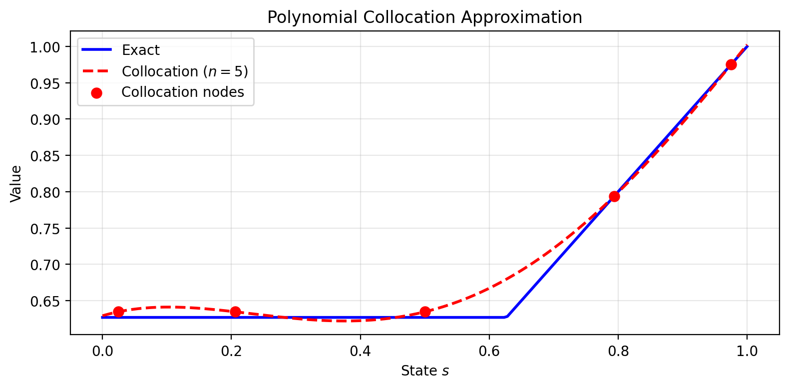
This example illustrates the fundamental tension in weighted residual methods: with finite parameters, we cannot satisfy the Bellman equation everywhere. We must choose how to allocate our approximation capacity. The rest of this chapter develops the general theory behind these choices.

Testing Whether a Residual Vanishes¶

Consider a functional equation $\Residual(f) = 0$, where $\Residual$ is an operator and the unknown $f$ is an entire function (in our case, the Bellman optimality equation $\Bellman v = v$, which we can write as $\Residual(v) \equiv \Bellman v - v = 0$). Suppose we have found a candidate approximate solution $\hat{f}$. To verify it satisfies $\Residual(\hat{f}) = 0$, we compute the residual function $R(s) = \Residual(\hat{f})(s)$. For a true solution, this residual should be the zero function: $R(s) = 0$ for every state $s$.

How might we test whether a function is zero? One approach: sample many input points $\{s_1, s_2, \ldots, s_m\}$, check whether $R(s_i) = 0$ at each, and summarize the results into a single scalar test by computing a weighted sum $\sum_{i=1}^m w_i R(s_i)$ with weights $w_i > 0$. If $R$ is zero everywhere, this sum is zero. If $R$ is nonzero somewhere, we can choose points and weights to make the sum nonzero. For vectors in finite dimensions, the inner product $\langle \mathbf{r}, \mathbf{y} \rangle = \sum_{i=1}^n r_i y_i$ implements exactly this idea: it tests $\mathbf{r}$ by weighting and summing. Indeed, a vector $\mathbf{r} \in \mathbb{R}^n$ equals zero if and only if $\langle \mathbf{r}, \mathbf{y} \rangle = 0$ for every vector $\mathbf{y} \in \mathbb{R}^n$. To see why, suppose $\mathbf{r} \neq \mathbf{0}$. Choosing $\mathbf{y} = \mathbf{r}$ gives $\langle \mathbf{r}, \mathbf{r} \rangle = \|\mathbf{r}\|^2 > 0$, contradicting the claim that all inner products vanish.

The same principle extends to functions. A function $R$ equals the zero function if and only if its “inner product” with every “test function” $p$ vanishes:

where $w(s) > 0$ is a weight function that is part of the inner product definition. Why does this work? For the same reason as in finite dimensions: if $R$ is not the zero function, there must be some region where $R(s) \neq 0$. We can then choose a test function $p$ that is nonzero in that same region (for instance, $p(s) = R(s)$ itself), which will produce $\langle R, p \rangle_w = \int R(s) p(s) w(s) ds > 0$, witnessing that $R$ is nonzero. Conversely, if $R$ is the zero function, then $\langle R, p \rangle_w = 0$ for any test function $p$.

This ability to distinguish between different functions using inner products is a fundamental principle from functional analysis. Just as we can test a vector by taking inner products with other vectors, we can test a function by taking inner products with other functions.

This transforms the pointwise condition “$R(s) = 0$ for all $s$” (infinitely many conditions, one per state) into an equivalent condition about inner products. We still cannot test against all possible test functions, since there are infinitely many of those too. But the inner product perspective suggests a natural computational strategy: choose a finite collection of test functions $\{p_1, \ldots, p_n\}$ and use them to construct $n$ conditions that we can actually compute.

From Variational Conditions to Optimization¶

Making a residual “small” is an optimization problem. We want to find $\theta$ that minimizes $\lVert R(\cdot; \theta) \rVert$ for some norm. Different methods correspond to different choices of norm:

• Minimize the weighted $L^2$ norm $\lVert R \rVert_w^2 = \int R(s)^2 w(s) ds$

• Minimize a discrete norm $\sum_j \omega_j R(s_j)^2$ at selected points

• Minimize $\lVert R \rVert$ in a dual norm induced by the approximation space

The first-order conditions for these optimization problems take the form $\langle R, p_j \rangle_w = 0$ for appropriate “test functions” $p_j$. The variational formulation is useful for analysis, but we are simply minimizing the residual in a chosen norm.

The rest of this chapter develops the computational framework: how to parameterize the unknown function, define the residual, choose a norm, and solve the resulting finite-dimensional problem.

The General Framework¶

Consider an operator equation of the form

where $\Residual: B_1 \to B_2$ is a continuous operator between complete normed vector spaces $B_1$ and $B_2$. For the Bellman equation, we have $\Residual(v) = \Bellman v - v$, so that solving $\Residual(v) = 0$ is equivalent to finding the fixed point $v = \Bellman v$.

Just as we transcribed infinite-dimensional continuous optimal control problems into finite-dimensional discrete optimal control problems in earlier chapters, we seek a finite-dimensional approximation to this infinite-dimensional functional equation. Recall that for continuous optimal control, we adopted control parameterization: we represented the control trajectory using a finite set of basis functions (piecewise constants, polynomials, splines) and searched over the finite-dimensional coefficient space instead of the infinite-dimensional function space. For integrals in the objective and constraints, we used numerical quadrature to approximate them with finite sums.

We follow the same strategy here. We parameterize the value function using a finite set of basis functions $\{\varphi_1, \ldots, \varphi_n\}$, commonly polynomials (Chebyshev, Legendre), though other function classes (splines, radial basis functions, neural networks) are possible, and search for coefficients $\theta = (\theta_1, \ldots, \theta_n)$ in $\mathbb{R}^n$. When integrals appear in the Bellman operator or projection conditions, we approximate them using numerical quadrature. The projection method approach consists of several conceptual steps that accomplish this transcription.

Step 1: Choose a Finite-Dimensional Approximation Space¶

We begin by selecting a basis $\Phi = \{\varphi_1, \varphi_2, \ldots, \varphi_n\}$ and approximating the unknown function as a linear combination:

The choice of basis functions $\varphi_i$ is problem-dependent. Common choices include:

• Polynomials: For smooth problems, we might use Chebyshev polynomials or other orthogonal polynomial families

• Splines: For problems where we expect the solution to have regions of different smoothness

• Radial basis functions: For high-dimensional problems where tensor product methods become intractable

The number of basis functions $n$ determines the flexibility of our approximation. In practice, we start with small $n$ and increase it until the approximation quality is satisfactory. The only unknowns now are the coefficients $\theta = (\theta_1, \ldots, \theta_n)$.

While the classical presentation of projection methods focuses on polynomial bases, the framework applies equally well to other function classes. Neural networks, for instance, can be viewed through this lens: a neural network $\hat{f}(x; \theta)$ with parameters $\theta$ defines a flexible function class, and many training procedures can be interpreted as projection methods with specific choices of test functions or residual norms. The distinction is that classical methods typically use predetermined basis functions with linear coefficients, while neural networks use adaptive nonlinear features. Throughout this chapter, we focus on the classical setting to develop the core concepts, but the principles extend naturally to modern function approximators.

Step 2: Define the Residual Function¶

Since we are approximating $f$ with $\hat{f}$, the operator $\Residual$ will generally not vanish exactly. Instead, we obtain a residual function:

This residual measures how far our candidate solution is from satisfying the equation at each point $x$. As we discussed in the introduction, we want to make this residual small—an optimization problem whose formulation depends on how we measure “small.”

Step 3: Minimize the Residual¶

Having chosen our basis and defined the residual, we must find $\theta$ that makes the residual small. This is an optimization problem: we minimize $\lVert R(\cdot; \theta) \rVert$ for some norm. The choice of norm determines the method:

The first-order conditions for each optimization problem yield $n$ equations in the $n$ unknowns $\theta_1, \ldots, \theta_n$. We now describe each method, starting with the most computationally attractive.

Collocation: Make the Residual Zero at Selected Points¶

The simplest approach is to choose $n$ points $\{x_1, \ldots, x_n\}$ and require the residual to vanish exactly at each:

This gives $n$ equations for $n$ unknowns. Collocation is computationally attractive because it avoids integration entirely—we only evaluate $R$ at discrete points. The resulting system is:

For a linear operator, this is a linear system; for the Bellman equation, it is nonlinear due to the max.

Verify for yourself: with $n = 2$ collocation points and $n = 2$ basis functions, the system $\boldsymbol{\Phi}\theta = t$ is a $2 \times 2$ linear system. What must be true about the collocation matrix $\boldsymbol{\Phi}$ for this system to have a unique solution?

The choice of collocation points matters. Orthogonal collocation (or spectral collocation) places points at the zeros of the $n$-th orthogonal polynomial in a family (Chebyshev, Legendre, etc.). For Chebyshev polynomials $T_0, T_1, \ldots, T_{n-1}$, we place collocation points at the zeros of $T_n(x)$. These points are also optimal nodes for Gauss quadrature, so:

• We get the computational simplicity of pointwise evaluation $R(x_i) = 0$

• When we need integrals (inside the Bellman operator), the collocation points double as quadrature nodes with exactness for polynomials up to degree $2n-1$

• For smooth problems, spectral approximations achieve exponential convergence: the error decreases like $O(e^{-cn})$ as we add basis functions, compared to $O(h^{p+1})$ for piecewise polynomials

The Chebyshev interpolation theorem guarantees that forcing $R(x_i; \theta) = 0$ at these carefully chosen points makes $R(x; \theta)$ small everywhere, with well-conditioned systems and near-optimal interpolation error.

Galerkin: Make the Residual Orthogonal to the Approximation Space¶

The Galerkin method requires the residual to be orthogonal to each basis function:

To understand why this is optimal, consider the approximation space $\mathcal{V} = \text{span}\{\varphi_1, \ldots, \varphi_n\}$ as an $n$-dimensional subspace. If the residual $R$ is orthogonal to all basis functions, then by linearity, $R$ is orthogonal to every function in $\mathcal{V}$:

The residual has “zero overlap” with our approximation space—it is as “invisible” to our basis as possible. This is the defining property of orthogonal projection.

In what sense is Galerkin minimizing a norm? The dual norm of $R$ with respect to $\mathcal{V}$ measures $R$ by its largest inner product with functions in $\mathcal{V}$:

The Galerkin conditions $\langle R, \varphi_j \rangle_w = 0$ for all $j$ imply $\langle R, g \rangle_w = 0$ for all $g \in \mathcal{V}$, so $\lVert R \rVert_{\mathcal{V}^*} = 0$. Galerkin makes the residual “invisible” when measured against the approximation space—it minimizes the dual norm to zero.

A finite-dimensional analogy: to approximate a vector $\mathbf{v} \in \mathbb{R}^3$ using only the $xy$-plane, the best approximation is $\hat{\mathbf{v}} = (v_1, v_2, 0)$. The error $\mathbf{r} = \mathbf{v} - \hat{\mathbf{v}} = (0, 0, v_3)$ points purely in the $z$-direction, orthogonal to the plane. The Galerkin condition generalizes this: the residual is orthogonal to the approximation space.

Galerkin requires integration to compute the conditions, making it more expensive per iteration than collocation. However, when using orthogonal polynomial bases with matching weight functions, the integrals simplify and the resulting systems are well-conditioned.

Least Squares: Minimize the $L^2$ Norm of the Residual¶

The most direct approach is to minimize the weighted $L^2$ norm of the residual:

The first-order conditions are:

This directly minimizes how far our approximation is from satisfying the equation. For the Bellman equation $R = \Bellman\hat{v} - \hat{v}$, this is Bellman residual minimization: we minimize $\lVert \Bellman\hat{v} - \hat{v} \rVert_w^2$.

The gradient $\frac{\partial R}{\partial \theta_j}$ involves differentiating the operator $\Residual$. For the Bellman operator with its max, this requires the Envelope Theorem (discussed in Step 4). The need to differentiate through the operator distinguishes least squares from Galerkin and collocation.

Fitted Q-Iteration: Project, Then Iterate¶

For iterative methods, there is a computationally simpler alternative to minimizing the residual directly. Fitted Q-Iteration (FQI) uses a two-step iteration:

1. Apply the Bellman operator to get a target: $f_k = \Bellman \hat{v}_k$

2. Project the target back onto the approximation space: $\hat{v}_{k+1} = \arg\min_\theta \lVert \hat{v}(\cdot; \theta) - f_k \rVert_w^2$

The projection step solves $\min_\theta \lVert \hat{v} - f_k \rVert_w^2$, whose first-order conditions are $\langle \hat{v} - f_k, \varphi_j \rangle_w = 0$. This is a standard least-squares fit of the basis to the target values. Combining these steps gives:

where $\Pi_w$ denotes orthogonal projection onto $\text{span}\{\varphi_j\}$ with respect to the weighted inner product.

FQI does not minimize the Bellman residual $\lVert \Bellman\hat{v} - \hat{v} \rVert^2$ directly. It projects, then iterates. FQI’s projection step uses only the gradient of $\hat{v}$ with respect to $\theta$ (the “semi-gradient”), while Bellman residual minimization requires differentiating through $\Bellman$ (the “full gradient”). We return to this distinction when discussing temporal difference learning.

Step 4: Solve the Finite-Dimensional Problem¶

The conditions from Step 3 give us a finite-dimensional problem to solve:

• Collocation: $n$ equations $R(x_i; \theta) = 0$

• Galerkin: $n$ equations $\int R(x; \theta) \varphi_i(x) w(x) dx = 0$

• Least squares: minimize $\int R(x; \theta)^2 w(x) dx$

In each case, we have $n$ equations (or first-order conditions) in $n$ unknowns $\theta_1, \ldots, \theta_n$. For the Bellman equation, these systems are nonlinear due to the max operator.

Computational Cost and Conditioning¶

The computational cost per iteration varies significantly across methods:

• Collocation: Cheapest to evaluate since $P_i(\theta) = R(x_i; \theta)$ requires only pointwise evaluation (no integration). The Jacobian is also cheap: $J_{ij} = \frac{\partial R(x_i; \theta)}{\partial \theta_j}$.

• Galerkin and moments: More expensive due to integration. Computing $P_i(\theta) = \int R(x; \theta) p_i(x) w(x) dx$ requires numerical quadrature. Each Jacobian entry requires integrating $\frac{\partial R}{\partial \theta_j} p_i w$.

• Least squares: Most expensive when done via the objective function, which requires integrating $R^2 w$. However, the first-order conditions reduce it to a system like Galerkin, with test functions $p_i = \partial R / \partial \theta_i$.

For methods requiring integration, the choice of quadrature rule should match the basis. Gaussian quadrature with nodes at orthogonal polynomial zeros is efficient. When combined with collocation at those same points, the quadrature is exact for polynomials up to a certain degree. This coordination between quadrature and collocation makes orthogonal collocation effective.

The conditioning of the system depends on the choice of test functions. The Jacobian matrix has entries:

When test functions are orthogonal (or nearly so), the Jacobian tends to be well-conditioned. This is why orthogonal polynomial bases are preferred in Galerkin methods: they produce Jacobians with controlled condition numbers. Poorly chosen basis functions or collocation points can lead to nearly singular Jacobians, causing numerical instability. Orthogonal bases and carefully chosen collocation points (like Chebyshev nodes) help maintain good conditioning.

Two Main Solution Approaches¶

We have two fundamentally different ways to solve the projection equations: function iteration (exploiting fixed-point structure) and Newton’s method (exploiting smoothness). The choice depends on whether the original operator equation has contraction properties and how well those properties are preserved by the finite-dimensional approximation.

Method 1: Function Iteration (Successive Approximation)¶

When the operator equation has the form $f = \Contraction f$ where $\Contraction$ is a contraction, the most natural approach is to iterate the operator directly:

The infinite-dimensional iteration becomes a finite-dimensional iteration in coefficient space once we choose our weighted residual method. Given a current approximation $\hat{f}^{(k)}(x; \theta^{(k)})$, how do we find the coefficients $\theta^{(k+1)}$ for the next iterate $\hat{f}^{(k+1)}$?

Different weighted residual methods answer this differently. For collocation, we proceed in two steps:

1. Evaluate the operator: At each collocation point $x_i$, compute what the next iterate should be: $t_i^{(k)} = (\Contraction \hat{f}^{(k)})(x_i)$. These $n$ target values tell us what $\hat{f}^{(k+1)}$ should equal at the collocation points.

2. Find matching coefficients: Determine $\theta^{(k+1)}$ so that $\hat{f}^{(k+1)}(x_i; \theta^{(k+1)}) = t_i^{(k)}$ for all $i$. This is a linear system: $\sum_j \theta_j^{(k+1)} \varphi_j(x_i) = t_i^{(k)}$.

In matrix form: $\boldsymbol{\Phi} \theta^{(k+1)} = t^{(k)}$, where $\boldsymbol{\Phi}$ is the collocation matrix with entries $\Phi_{ij} = \varphi_j(x_i)$. Solving this system gives $\theta^{(k+1)} = \boldsymbol{\Phi}^{-1} t^{(k)}$.

For Galerkin, the projection condition $\langle \hat{f}^{(k+1)} - \Contraction \hat{f}^{(k+1)}, \varphi_i \rangle_w = 0$ directly gives a system for $\theta^{(k+1)}$. When $\Contraction$ is linear in its argument (as in many integral equations), this is a linear system. When $\Contraction$ is nonlinear (as in the Bellman equation), we must solve a nonlinear system at each iteration, though each solution still only involves $n$ unknowns rather than an infinite-dimensional function.

When $\Contraction$ is a contraction in the infinite-dimensional space with constant $\gamma < 1$, iterating it pulls any starting function toward the unique fixed point. The hope is that the finite-dimensional operator, evaluating $\Contraction$ and projecting back onto the span of the basis functions, inherits this contraction property. When it does, function iteration converges globally from any initial guess, with each iteration reducing the error by a factor of roughly $\gamma$. This is computationally attractive: we only evaluate the operator and solve a linear system (for collocation) or a relatively simple system (for other methods).

However, the finite-dimensional approximation doesn’t always preserve contraction. High-order polynomial bases, in particular, can create oscillations between basis functions that amplify rather than contract errors. Even when contraction is preserved, convergence can be painfully slow when $\gamma$ is close to 1, the “weak contraction” regime common in economic problems with patient agents ($\gamma \approx 0.95$ or higher). Finally, not all operator equations naturally present themselves as contractions; some require reformulation (like $f = f - \alpha \Residual(f)$), and finding a good $\alpha$ can be problem-specific.

Method 2: Newton’s Method¶

Alternatively, we can treat the projection equations as a rootfinding problem $G(\theta) = 0$ where $G_i(\theta) = P_i(\theta)$ for test function methods, or solve the first-order conditions for least squares. Newton’s method uses the update:

where $J_G(\theta)$ is the Jacobian of $G$ at $\theta$.

To apply this update, we must compute the Jacobian entries $J_{ij} = \frac{\partial G_i}{\partial \theta_j}$. For collocation, $G_i(\theta) = \hat{f}(x_i; \theta) - (\Contraction \hat{f}(\cdot; \theta))(x_i)$, so:

The first term is straightforward (it’s just $\varphi_j(x_i)$ for a linear approximation). The second term requires differentiating the operator $\Contraction$ with respect to the parameters.

When $\Contraction$ involves optimization (as in the Bellman operator $\Bellman v = \max_a \{r(s,a) + \gamma \mathbb{E}[v(s')]\}$), computing this derivative appears problematic because the max operator is not differentiable. However, the Envelope Theorem resolves this difficulty.

Before reading the box below, try differentiating $v(\theta) = \max_x f(x, \theta)$ using the chain rule. What term involving $\partial x^*/\partial \theta$ appears? Why might this term vanish at an optimum?

With the Envelope Theorem providing a tractable way to compute Jacobians for problems involving optimization, Newton’s method becomes practical for weighted residual methods applied to Bellman equations and similar problems. The method offers quadratic convergence near the solution. Once in the neighborhood of the true fixed point, Newton’s method typically converges in just a few iterations. Unlike function iteration, it doesn’t rely on the finite-dimensional approximation preserving any contraction property, making it applicable to a broader range of problems, particularly those with high-order polynomial bases or large discount factors where function iteration struggles.

However, Newton’s method demands more from both the algorithm and the user. Each iteration requires computing and solving a full Jacobian system, making the per-iteration cost significantly higher than function iteration. The method is also sensitive to initialization: started far from the solution, Newton’s method may diverge or converge to spurious fixed points that the finite-dimensional problem introduces but the original infinite-dimensional problem lacks. When applying the Envelope Theorem, implementation becomes more complex. We must track the optimal action at each evaluation point and compute the Jacobian entries using the formula above (expected basis function values at next states under optimal actions), though the economic interpretation (tracking how value propagates through optimal decisions) often makes the computation conceptually clearer than explicit derivative calculations would be.

Comparison and Practical Recommendations¶

Which method to use? When the problem has strong contraction (small $\gamma$, well-conditioned bases, shape-preserving approximations like linear interpolation or splines), function iteration is simple and robust. For weak contraction (large $\gamma$, high-order polynomials), a hybrid approach works well: run function iteration for several iterations to enter the basin of attraction, then switch to Newton’s method for rapid final convergence. When the finite-dimensional approximation destroys contraction entirely (common with non-monotone bases), Newton’s method may be necessary from the start, though careful initialization (from a coarser approximation or perturbation methods) is required.

Quasi-Newton methods like BFGS or Broyden offer a middle ground. They approximate the Jacobian using function evaluations only, avoiding explicit derivative computations while maintaining superlinear convergence. This can be useful when computing the exact Jacobian via the Envelope Theorem is expensive or when the approximation quality is acceptable.

Step 5: Verify the Solution¶

Once we have computed a candidate solution $\hat{f}$, we must verify its quality. Projection methods optimize $\hat{f}$ with respect to specific criteria (specific test functions or collocation points), but we should check that the residual is small everywhere, including directions or points we did not optimize over.

Typical diagnostic checks include:

• Computing $\|R(\cdot; \theta)\|$ using a more accurate quadrature rule than was used in the optimization

• Evaluating $R(x; \theta)$ at many points not used in the fitting process

• If using Galerkin with the first $n$ basis functions, checking orthogonality against higher-order basis functions

In summary, we have established a template: parameterize the unknown function using basis functions, define a residual measuring how far from a solution we are, and impose conditions via inner products with test functions. Different test functions yield different methods: Galerkin uses the basis itself, collocation uses delta functions at chosen points, and least squares uses residual gradients. We now apply this framework to the Bellman equation.

Application to the Bellman Equation¶

Consider the Bellman optimality equation $v(s) = \Bellman v(s) = \max_{a \in \mathcal{A}_s} \{ r(s,a) + \gamma \sum_{j \in \mathcal{S}} p(j|s,a) v(j) \}$. For a candidate approximation $\hat{v}(s) = \sum_{i=1}^n \theta_i \varphi_i(s)$, the residual is:

We examine how collocation and Galerkin, the two most common weighted residual methods for Bellman equations, specialize the general solution approaches from Step 4.

Collocation¶

For collocation, we choose $n$ states $\{s_1, \ldots, s_n\}$ and require the Bellman equation to hold exactly at these points:

It helps to define the parametric Bellman operator $\mathrm{L}_\varphi: \mathbb{R}^n \to \mathbb{R}^n$ by $[\mathrm{L}_\varphi(\theta)]_i = [\Bellman\hat{v}(\cdot; \theta)](s_i)$, the Bellman operator evaluated at collocation point $s_i$. Let $\boldsymbol{\Phi}$ be the $n \times n$ matrix with entries $\Phi_{ij} = \varphi_j(s_i)$. Then the collocation equations become $\boldsymbol{\Phi} \theta = \mathrm{L}_\varphi(\theta)$.

Function iteration for collocation proceeds as follows. Given current coefficients $\theta^{(k)}$, we evaluate the Bellman operator at each collocation point to get target values $t_i^{(k)} = [\mathrm{L}_\varphi(\theta^{(k)})]_i$. We then find new coefficients by solving the linear system $\boldsymbol{\Phi} \theta^{(k+1)} = t^{(k)}$. This is parametric value iteration: apply the Bellman operator, fit the result.

When the state space is continuous, we approximate expectations using numerical quadrature (Gauss-Hermite for normal shocks, etc.). The method is simple and robust when the finite-dimensional approximation preserves contraction, but can be slow for large discount factors.

Newton’s method for collocation treats the problem as rootfinding: $G(\theta) = \boldsymbol{\Phi} \theta - \mathrm{L}_\varphi(\theta) = 0$. The Jacobian is $J_G = \boldsymbol{\Phi} - J_{\mathrm{L}_\varphi}$, where the Envelope Theorem (Step 4) gives us $[J_{\mathrm{L}_\varphi}]_{ij} = \gamma \sum_{s'} p(s'|s_i, a_i^*(\theta)) \varphi_j(s')$. Here $a_i^*(\theta)$ is the optimal action at collocation point $s_i$ given the current coefficients.

This converges rapidly near the solution but requires good initialization and more computation per iteration than function iteration. The method is equivalent to policy iteration: each step evaluates the value of the current greedy policy, then improves it.

Why is collocation popular for Bellman equations? Because it avoids integration when testing the residual. We only evaluate the Bellman operator at $n$ discrete points. In contrast, Galerkin requires integrating the residual against each basis function.

Worked Example: Collocation on the Optimal Stopping Problem¶

Returning to our motivating example, let us trace through the collocation algorithm with $n = 4$ polynomial basis functions at Chebyshev nodes:

import numpy as np
from scipy.integrate import quad

gamma = 0.9
n = 4

# Chebyshev nodes on [0, 1]
k = np.arange(1, n + 1)
nodes = 0.5 + 0.5 * np.cos((2*k - 1) * np.pi / (2*n))
nodes = np.sort(nodes)

# Vandermonde matrix
Phi = np.vander(nodes, n, increasing=True)

# Exact solution
v_bar_exact = (1 - np.sqrt(1 - gamma**2)) / gamma**2
s_star_exact = gamma * v_bar_exact
def v_exact(s):
    return np.where(s >= s_star_exact, s, gamma * v_bar_exact)

# Collocation iteration
theta = np.zeros(n)
print("Collocation iteration trace:")
print(f"{'Iter':<6} {'||theta||':<12} {'Max error':<12}")
print("-" * 30)

for iteration in range(15):
    def v_approx(s, th=theta):
        return sum(th[j] * s**j for j in range(n))
    v_bar, _ = quad(v_approx, 0, 1)
    test_points = np.linspace(0, 1, 100)
    max_error = max(abs(v_approx(s) - v_exact(s)) for s in test_points)
    print(f"{iteration:<6} {np.linalg.norm(theta):<12.6f} {max_error:<12.6f}")
    
    targets = np.maximum(nodes, gamma * v_bar)
    theta_new = np.linalg.solve(Phi, targets)
    if np.linalg.norm(theta_new - theta) < 1e-10:
        print(f"\nConverged in {iteration + 1} iterations")
        break
    theta = theta_new

Collocation iteration trace:
Iter   ||theta||    Max error   
------------------------------
0      0.000000     1.000000    
1      1.000000     0.626789    
2      1.613062     0.198576    
3      0.706118     0.087935    
4      1.044850     0.039335    
5      1.292433     0.032162    
6      1.412062     0.033449    
7      1.467070     0.034028    
8      1.492030     0.034289    
9      1.503301     0.034406    
10     1.508381     0.034459    
11     1.510668     0.034483    
12     1.511698     0.034493    
13     1.512161     0.034498    
14     1.512370     0.034500    

Galerkin¶

For Galerkin, we use the basis functions themselves as test functions. The conditions are:

where $w(s)$ is a weight function (often the stationary distribution $d^\pi(s)$ in RL applications, or simply $w(s) = 1$). Expanding this:

Function iteration for Galerkin works differently than for collocation. Given $\theta^{(k)}$, we cannot simply evaluate the Bellman operator and fit. Instead, we must solve an integral equation. At each iteration, we seek $\theta^{(k+1)}$ satisfying:

The left side is a linear system (the “mass matrix” $M_{ij} = \int \varphi_i \varphi_j w$), and the right side requires integrating the Bellman operator output against each test function. When the basis functions are orthogonal polynomials with matching weight $w$, the mass matrix is diagonal, simplifying the solve. But we still need numerical integration to evaluate the right side. This makes Galerkin substantially more expensive than collocation per iteration.

Newton’s method for Galerkin similarly requires integration. The residual is $R(s; \theta) = \Bellman\hat{v}(s; \theta) - \hat{v}(s; \theta)$, and we need $G_i(\theta) = \int R(s; \theta) \varphi_i(s) w(s) ds = 0$. The Jacobian entry is:

The Envelope Theorem gives $\frac{\partial \Bellman\hat{v}(s; \theta)}{\partial \theta_j} = \gamma \mathbb{E}[\varphi_j(s') \mid s, a^*(s;\theta)]$, so we must integrate expected basis function values (under optimal actions) against test functions and weight. This requires both numerical integration and careful tracking of optimal actions across the state space, making it substantially more complex than collocation’s pointwise evaluation.

The advantage of Galerkin over collocation lies in its theoretical properties: when using orthogonal polynomials, Galerkin provides optimal approximation in the weighted $L^2$ norm. For smooth problems, this can yield better accuracy per degree of freedom than collocation. In practice, collocation’s computational simplicity usually outweighs Galerkin’s theoretical optimality for Bellman equations, especially in high-dimensional problems where integration becomes prohibitively expensive.

The algorithms above reduce the infinite-dimensional Bellman fixed-point problem to finite-dimensional coefficient computation. Collocation avoids integration entirely by requiring exact satisfaction at discrete points, while Galerkin imposes weighted orthogonality conditions requiring numerical quadrature. Both can be solved via function iteration (when contraction is preserved) or Newton’s method (for faster convergence near the solution). The discrete MDP specialization below reveals connections to algorithms widely used in reinforcement learning.

Galerkin for Discrete MDPs: LSTD and LSPI¶

When the state space is discrete and finite, the Galerkin conditions simplify dramatically. The integrals become sums, and we can write everything in matrix form. This specialization shows the connection to algorithms widely used in reinforcement learning.

For a discrete state space $\mathcal{S} = \{s_1, \ldots, s_m\}$, the Galerkin orthogonality conditions

become weighted sums over states:

where $\xi(s) \geq 0$ with $\sum_s \xi(s) = 1$ is a probability distribution over states. Define the feature matrix $\boldsymbol{\Phi} \in \mathbb{R}^{m \times n}$ with entries $\Phi_{si} = \varphi_i(s)$ (each row contains the features for one state), and let $\boldsymbol{\Xi} = \text{diag}(\xi)$ be the diagonal matrix with the state distribution on the diagonal.

Policy Evaluation: LSTD¶

For policy evaluation with a fixed policy $\pi$, the Bellman operator is linear:

With linear function approximation $\hat{v}(s) = \boldsymbol{\varphi}(s)^\top \theta = \sum_i \theta_i \varphi_i(s)$, this becomes:

Let $\mathbf{r}_\pi \in \mathbb{R}^m$ be the vector of rewards $[\mathbf{r}_\pi]_s = r(s, \pi(s))$, and $\mathbf{P}_\pi \in \mathbb{R}^{m \times m}$ be the transition matrix with $[\mathbf{P}_\pi]_{sj} = p(j|s, \pi(s))$. Then $\BellmanPi \hat{v} = \mathbf{r}_\pi + \gamma \mathbf{P}_\pi \boldsymbol{\Phi} \theta$ in vector form.

The Galerkin conditions require $\langle \BellmanPi \hat{v} - \hat{v}, \varphi_i \rangle_\xi = 0$ for all basis functions, which in matrix form is:

Rearranging:

This is the LSTD (Least Squares Temporal Difference) solution. The matrix $\mathbf{A} = \boldsymbol{\Phi}^\top \boldsymbol{\Xi} (\boldsymbol{\Phi} - \gamma \mathbf{P}_\pi \boldsymbol{\Phi})$ and vector $\mathbf{b} = \boldsymbol{\Phi}^\top \boldsymbol{\Xi} \mathbf{r}_\pi$ give the linear system $\mathbf{A} \theta = \mathbf{b}$.

When $\xi$ is the stationary distribution of policy $\pi$ (so $\xi^\top \mathbf{P}_\pi = \xi^\top$), this system has a unique solution, and the projected Bellman operator $\Proj \BellmanPi$ is a contraction in the weighted $L^2$ norm $\|\cdot\|_\xi$. This is the theoretical foundation for TD learning with linear function approximation. The fixed point computed here is the same one that TD(0) converges to stochastically; we derive the incremental algorithm in the Monte Carlo chapter.

Check that the dimensions work out: if we have $m$ states and $n$ basis functions, what are the dimensions of $\boldsymbol{\Phi}$, $\boldsymbol{\Xi}$, $\mathbf{P}_\pi$, and the matrix $\mathbf{A} = \boldsymbol{\Phi}^\top \boldsymbol{\Xi}(\boldsymbol{\Phi} - \gamma \mathbf{P}_\pi \boldsymbol{\Phi})$?

Worked Example: LSTD for Policy Evaluation¶

To illustrate LSTD concretely, consider a 3-state Markov chain under a fixed policy:

import numpy as np

P_pi = np.array([[0.7, 0.2, 0.1], [0.3, 0.4, 0.3], [0.1, 0.3, 0.6]])
r_pi = np.array([1.0, 2.0, 0.0])
gamma = 0.9

# Feature matrix: phi_1(s) = 1, phi_2(s) = s
states = np.array([1, 2, 3])
Phi = np.column_stack([np.ones(3), states])

# Uniform weighting
xi = np.ones(3) / 3
Xi = np.diag(xi)

# LSTD matrices
A = Phi.T @ Xi @ (Phi - gamma * P_pi @ Phi)
b = Phi.T @ Xi @ r_pi

theta_lstd = np.linalg.solve(A, b)
v_lstd = Phi @ theta_lstd
v_exact = np.linalg.solve(np.eye(3) - gamma * P_pi, r_pi)

print(f"LSTD solution: theta = ({theta_lstd[0]:.4f}, {theta_lstd[1]:.4f})")
print(f"\n{'State':<8} {'Exact':<12} {'LSTD':<12} {'Error':<12}")
print("-" * 44)
for s in range(3):
    print(f"{s+1:<8} {v_exact[s]:<12.4f} {v_lstd[s]:<12.4f} {v_lstd[s] - v_exact[s]:<12.4f}")

# Verify orthogonality
residual = r_pi + gamma * P_pi @ v_lstd - v_lstd
print(f"\nGalerkin orthogonality: <residual, phi_1> = {np.sum(xi * residual * Phi[:,0]):.6f}")

LSTD solution: theta = (12.2772, -0.9901)

State    Exact        LSTD         Error       
--------------------------------------------
1        10.0207      11.2871      1.2664      
2        10.8717      10.2970      -0.5746     
3        8.3418       9.3069       0.9652      

Galerkin orthogonality: <residual, phi_1> = 0.000000

The Bellman Optimality Equation: Function Iteration and Newton’s Method¶

For the Bellman optimality equation, the max operator introduces nonlinearity:

The Galerkin conditions become:

where the Bellman operator must be evaluated at each state $s$ to find the optimal action and compute the target value. This is a system of $n$ nonlinear equations in $n$ unknowns.

Function iteration applies the Bellman operator and projects back. Given $\theta^{(k)}$, compute the greedy policy $\pi^{(k)}(s) = \arg\max_a \{r(s,a) + \gamma \sum_{j \in \mathcal{S}} p(j|s,a) \boldsymbol{\varphi}(j)^\top \theta^{(k)}\}$ at each state, then solve:

This evaluates the current greedy policy using LSTD, then implicitly improves by computing a new greedy policy at the next iteration. However, convergence can be slow when the finite-dimensional approximation poorly preserves contraction.

Newton’s method treats $G(\theta) = 0$ as a rootfinding problem and uses the Jacobian to accelerate convergence. The Jacobian of $G$ is:

To compute $\frac{\partial \Bellman\hat{v}(s; \theta)}{\partial \theta_j}$, we use the Envelope Theorem from Step 4. At the current $\theta^{(k)}$, let $a^*(s; \theta^{(k)})$ be the optimal action at state $s$. Then:

Define the policy $\pi^{(k)}(s) = a^*(s; \theta^{(k)})$. The Jacobian becomes:

The Newton update $\theta^{(k+1)} = \theta^{(k)} - J_G(\theta^{(k)})^{-1} G(\theta^{(k)})$ simplifies. We have:

At each state $s$, the greedy value is $[\Bellman\hat{v}(\cdot; \theta^{(k)})](s) = r(s, \pi^{(k)}(s)) + \gamma \sum_j p(j|s, \pi^{(k)}(s)) \boldsymbol{\varphi}(j)^\top \theta^{(k)}$, which equals $[\mathrm{L}_{\pi^{(k)}} \hat{v}(\cdot; \theta^{(k)})](s)$. Thus:

The Newton step becomes:

Multiplying through and simplifying:

This is LSPI (Least Squares Policy Iteration). Each Newton step:

1. Computes the greedy policy $\pi^{(k)}(s) = \arg\max_a \{r(s,a) + \gamma \sum_j p(j|s,a) \boldsymbol{\varphi}(j)^\top \theta^{(k)}\}$

2. Solves the LSTD equation for this policy to get $\theta^{(k+1)}$

Newton’s method for the Galerkin-projected Bellman optimality equation is equivalent to policy iteration in the function approximation setting. Just as Newton’s method for collocation corresponded to policy iteration (Step 4), Newton’s method for discrete Galerkin gives LSPI.

Galerkin projection with linear function approximation reduces policy iteration to a sequence of linear systems, each solvable in closed form. For discrete MDPs, we can compute the matrices $\boldsymbol{\Phi}^\top \boldsymbol{\Xi} \boldsymbol{\Phi}$ and $\boldsymbol{\Phi}^\top \boldsymbol{\Xi} \mathbf{P}_\pi \boldsymbol{\Phi}$ exactly.

Extension to Nonlinear Approximators¶

The weighted residual methods developed so far have focused on linear function classes: polynomial bases, piecewise linear interpolants, and linear combinations of fixed basis functions. Neural networks, kernel methods, and decision trees do not fit this template. How does the framework extend to nonlinear approximators?

Recall the Galerkin approach for linear approximation $v_{\boldsymbol{\theta}} = \sum_{i=1}^d \theta_i \varphi_i$. The orthogonality conditions $\langle v - \Bellman v, \varphi_i \rangle_w = 0$ for all $i$ define a linear system with a closed-form solution. These equations arise from minimizing $\|v - \Bellman v\|_w^2$ over the subspace, since at the minimum, the gradient with respect to each coefficient must vanish. The connection between norm minimization and orthogonality holds generally. For any norm $\|\cdot\|_w$ induced by an inner product $\langle \cdot, \cdot \rangle_w$, minimizing $\|f(\boldsymbol{\theta})\|_w^2$ with respect to parameters requires $\frac{\partial}{\partial \theta_i} \|f(\boldsymbol{\theta})\|_w^2 = 0$. Since $\|f\|_w^2 = \langle f, f \rangle_w$, the chain rule gives $2\langle f, \frac{\partial f}{\partial \theta_i} \rangle_w = 0$. Minimizing the residual norm is thus equivalent to requiring orthogonality $\langle f, \frac{\partial f}{\partial \theta_i} \rangle_w = 0$ for all $i$. The equivalence holds for any choice of inner product: weighted $L^2$ integrals for Galerkin, sums over collocation points for collocation, or sampled expectations for neural networks.